An algorithm for generation of DEMs from contour lines considering geomorphic features

Geomorphic information is omitted from many existing methods of generating gridded digital elevation models (DEMs) from contour lines, resulting in significant errors during interpolation. Here, we present an advanced schema for improvement of the comprehensive regionalized method of linear interpolation. This approach uses a moving fitting method for an interpolated point and selects elevation points that are representative of geomorphic features as a whole to improve interpolation quality. A total of 16 points are selected, according to certain criteria, in eight directions surrounding the interpolated point; thus, there are two points in each direction, which is sufficient to provide an accurate representation of the geomorphic features of the DEM. Our method introduces virtual control points to prevent sudden changes in the interpolation results, which helps to overcome problems related to the distortion of the local geospatial distribution in areas where feature geomorphic information is inadequate. We construct the spline interpolation function using intersection points and virtual control points, all of which are applied to compute the point elevation. Moreover, we index all elevation values and spatial points of linear features using the R-tree method to ensure that points related to an interpolated position can be retrieved as quickly as possible. Finally, we test our method using a coal mine elevation dataset. The results confirm that our proposed method can generate DEMs smoothly and, in particular, avoid problems related to local distortion. 

Resumen

La información geomórfica se omite en muchos de los métodos de generación de Modelos Digitales de Elevación (DEM, en inglés) que se elaboran a partir de líneas de contorno, lo que resulta en errores significativos durante la interpolación. En este trabajo se presenta un esquema avanzado para el mejoramiento del método comprensivo regionalizado de interpolación lineal. Esta aproximación utiliza un método de ajuste móvil para un punto interpolado y selecciona puntos de elevación representativos o características geomórficas como un todo para mejorar la calidad de la interpolación. Se seleccionaron 16 puntos de acuerdo con ciertos criterios, en ocho direcciones alrededor del punto interpolado; por lo tanto, hay dos puntos en cada dirección, lo que es suficiente para proveer una representación precisa de las características geomórficas del DEM. El método propuesto consta de puntos virtuales de control para prevenir cambios repentinos en los resultados de la interpolación, lo que ayuda a vencer los problemas relacionados a la distorsión de la distribución geoespacial local en áreas donde la información de las características geomórficas es inadecuada. Se utilizó una función de interpolación spline con puntos de intersección y puntos de control virtual, que fueron utilizados para calcular el punto de elevación. Además, se indexaron todos los valores de elevación y los puntos espaciales de las características lineales con el método de árbol-R para asegurar que los puntos relacionados a una posición interpolada pueden ser recuperados tan rápido como sea posible. Finalmente, el método fue evaluado con la configuración de elevación de una mina de carbón. Los resultados confirman que el método propuesto puede generar modelos sin problemas y, en particular, evitar complicaciones relacionadas a distorsión local. 

Doi: https://doi.org/10.15446/esrj.v20n2.55348

Algoritmo para la generación de Modelos Digitales de Elevación considerando líneas de contorno y características geomórficas

Xiao-Ping Rui¹, Xue-Tao Yu^{2, 3}, Jin Lu⁴, Muhammad Aqeel Ashraf⁵, Xian-Feng Song^1*

¹ College of Resources and Environment, University of Chinese Academy of Sciences, Beijing 100049, China;
² School of Traffic and Transportation, Shijiazhuang Tiedao University, Shijiazhuang 050043, China;
³ Traffic Safety and Control Lab in Hebei Province, Shijiazhuang 050043, China;
⁴ China Institute of Water Resources and Hydropower Research, Beijing 100038, China;
⁵ Faculty of Science and Natural Resurces, University Malaysia Sabah 88400 Kota Kinabalu, Sabah, Malaysia;
* Corresponding author, email: song7537338@163.com

Record
Manuscript received: 25/01/2016 Accepted for publication: 15/07/2016

How to cite item
Rui, X. P., Yu, X. T., Lu, J., Ashraf, M. A., & Song, X. F. (2016). An algorithm for generation of DEMs from contour lines considering geomorphic features. Earth Sciences Research Journal, 20(2), G1-G9. doi: https://doi.org/10.15446/esrj.v20n2.55348

---

ABSTRACT

Keywords: Digital Elevation Models (DEM), interpolation points, contour lines map, geomorphic features.

---

La información geomórfica se omite en muchos de los métodos de generación de Modelos Digitales de Elevación (DEM, en inglés) que se elaboran a partir de líneas de contorno, lo que resulta en errores significativos durante la interpolación. En este trabajo se presenta un esquema avanzado para el mejoramiento del método comprensivo regionalizado de interpolación lineal. Esta aproximación utiliza un método de ajuste movil para un punto interpolado y selecciona puntos de elevación representativos o características geomórficas como un todo para mejorar la calidad de la interpolación. Se seleccionaron 16 puntos de acuerdo con ciertos criterios, en ocho direcciones alrededor del punto interpolado; por lo tanto, hay dos puntos en cada dirección, lo que es suficiente para proveer una representación precisa de las características geomórficas del DEM. El método propuesto consta de puntos virtuales de control para prevenir cambios repentinos en los resultados de la interpolación, lo que ayuda a vencer los problemas relacionados a la distorsión de la distribución geoespacial local en áreas donde la información de las características geomórficas es inadecuada. Se utilizó una función de interpolación spline con puntos de intersección y puntos de control virtual, que fueron utilizados para calcular el punto de elevación. Además, se indexaron todos los valores de elevación y los puntos espaciales de las características lineales con el método de árbol-R para asegurar que los puntos relacionados a una posición interpolada pueden ser recuperados tan rápido como sea posible. Finalmente, el método fue evaluado con la configuración de elevación de una mina de carbón. Los resultados confirman que el método propuesto puede generar modelos sin problemas y, en particular, evitar complicaciones relacionadas a distorsión local.

Palabras clave: Modelos de Evaluación Digital, puntos de interpolación, mapas lineales de contorno, características geomórficas.

---

1. Introduction

Digital elevation models (DEMs) are imperative in the field of geosciences and have been used widely in the generation and display of three-dimensional terrain. For example, DEMs have been applied to investigate slope and aspect, construct terrain profiles between selected points, and delineate other significant surface features (Kweon and Kanade, 1994; Zhou and Liu, 2004; Zhou and Chen, 2011; Hickey et al., 1994; Jones, 1998; Oky et al., 2002). Many methods have been proposed to generate DEM data, including photogrammetry techniques, radar interferometry, laser altimetry, and interpolation (Wood and Fisher, 1993; Wood, 1994; Hearnshaw and Unwin, 1994). Although elevation mapping technology now allows production of DEMs directly from measured points, accurate interpolation from contours is still important in areas where high-resolution DEMs are not available (Taud et al., 1999; Werbrouck et al., 2011) or in cases where historical contour maps are used to evaluate topographic change (Carley et al., 2012). For the generation of regional or continental DEMs, interpolation methods using fine scale contours are useful owing to their low cost and the relative ease of obtaining contour maps in this way (Doytsher and Hall, 1997; Heritage et al., 2009; Wise, 2011).

Accordingly, various interpolation algorithms have been developed to generate DEMs from contours. The contours, which are in vector or raster format, consist of a large number of elevation points. Moreover, the shape of (and geometric relationships between) the contours can be indicative of certain geomorphic features. To determine the elevation at a given point, interpolation algorithms often adopt a sampling strategy that selects representative elevation points from contours in order to reduce computation time, subsequently conducting interpolation using functions such as the inverse distance weight function or surface spline function (Huang et al., 2011; Maekawa et al., 2007; Gofuku et al., 2009). Here, we describe several of the most popular interpolation algorithms.

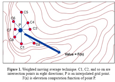
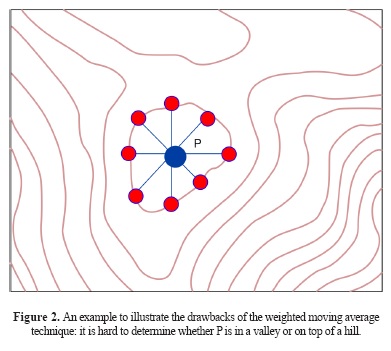
The weighted moving average technique interpolates by making use of the geometric relationships between adjacent contour lines (Watson, 1992). For a given grid, the elevation at each cell is computed as follows. First, geometrical rays are drawn from the cell center following both cardinal and intermediate directions. Then, eight corresponding intersection points between those rays and their closest adjacent contour lines are identified, and the elevation value F(n) is computed from these intersection points using the inverse distance weight method (Figure 1) based on these eight crossing points (C1, C2… C8). However, this approach cannot reflect the topography of mountaintops and depressions with sufficient resolution for most purposes (Figure 2) (Rvachev et al., 2001; Dinis et al., 2007; Watson, 1999).

Taud et al. (1999) developed a raster-based interpolation method to generate digital elevation models through the dilation of contour lines stored in a raster grid. This method uses an iterative procedure to produce an extension of contour lines by applying alternate four- and eight-connected erosions of the background until the generated surfaces become contiguous. This process stops when no new contour lines can be generated. The contour line dilation algorithm can prevent any crossing, especially when the isoline contours are adjacent. This method is simple to apply and has a low computational cost (Oky et al., 2002; Gousie and Franklin, 2003). However, it is clear that, when the contour line is closed, the interpolated data in the inner exhibits the same elevation value as the closed contour line, which may result in error.

To insert the height of steep slope areas, Xie et al. (2003) developed a special kernel filter that can interpolate a grid cell through which multiple contour lines pass. The contour lines are first rasterized as a grid. Then, three cell types are defined concerning the relationships between contours and cells: no-value (NVC), single-value (SVC), and multi-value (MVC) cells, which indicate no contour lines, a single contour line, or multiple contour lines passing through the cell, respectively. The elevations of MVCs are computed using an MVC filter, whereas those of SVCs are directly assigned based on the appropriate contour elevation. The value of a given NVC is interpolated from its neighboring SVCs or MVCs in both the cardinal and intermediate directions. Wang et al. (2005) further improved the interpolation of the elevation of SVCs by considering the spatial relationship between SVC-associated contours and their neighboring contours. In this modified method, a triangulated irregular network is constructed using two adjacent contours; then, the triangle within which the SVC center falls is identified and its three vertices used to interpolate the elevation of the SVC.

Clarke et al. (1982) evaluated three interpolation methods: linear interpolation with four data points found in the grid axis directions (LIXY), linear interpolation between two data points found in the approximate direction of steepest slope (LISS), and cubic interpolation using four data points found in the approximate direction of steepest slope (CISS). Their results indicated that DEMs generated using methods that consider terrain features such as break lines, ridges, and spot heights are more accurate than those generated using methods that do not take such features into account. However, the methods introduced by Clarke et al. (1982) use only a few points to infer geomorphic trends; thus, they are successful in improving the quality of DEMs but are incapable of delineating specific patterns.

Skeleton lines (i.e., ridge and drainage lines) are essential for the description of terrain surfaces. Aumann et al. (1991) developed two methods to achieve automatic derivation of skeleton lines from digitized contours but were unable to apply their results to generate DEMs from contours. Conversely, a hydrologically correct grid of elevation can be produced using Hutchinson's algorithm, which takes into account information inherent to the contours and uses them to build a generalized drainage model. Then, this information can be applied to form constraints for the interpolation process to ensure that the output DEM displays appropriate hydrogeomorphic properties (Hutchinson 1988, 1996, 2008). Using this method, a network of streams and ridges can be built by identifying areas of local maximum curvature in each contour and, thus, the field of steepest slope. The interpolation procedure uses a discretized thin plate spline technique, where the roughness penalty has been modified to allow the fitted DEM to follow abrupt changes in terrain (e.g., streams and ridges). The method uses a maximum of 50 data points from these contours within each cell, which improves computational efficiency. This algorithm has a well-known implementation of TOPOGRID in ArcGIS, and the drainage conditions imposed by the algorithm produce higher accuracy surfaces with fewer input data (Peralvo and Maident, 2008; Binh and Thuy, 2008).

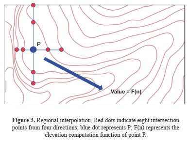
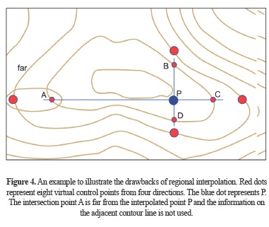
To enable interpolation in the regions surrounding mountaintops or depressions, Yu and Tan (2002) proposed a regionalized comprehensive interpolation method to produce DEMs using contour lines. Based on an interpolated point, geometrical rays in the horizontal and vertical directions are used to intersect with two neighboring contour lines, thus producing a total of eight intersection points in four directions (Figure 3). These intersection points are then used to calculate the point elevation using a surface spline function (Yu, 2001). This system represents a considerable advantage over the above methods, in that the method of Yu and Tan (2002) can predict the elevations of mountaintops or depressions using splines because the sample points along each ray direction have different height values. However, points obtained from only four fixed cardinal directions may not be representative; that is, the points on contour lines that are close to the interpolated cell may not be selected, but the points obtained from the intersection points between contour lines and rays that are far from the interpolated cell are selected (Figure 4). Thus, this method often leads to serious errors, particularly in narrow ridge or valley areas with steep slopes or cliffs.

The quality of the derived DEM depends greatly on the data source and interpolation technique used (Heritage et al., 2009; Bouillon et al., 2006; Wise, 2011, 2012). Vieux (1993) was the first to suggest that the Shannon–Weaver information statistic, often referred to as entropy, might offer potential as a measure of some characteristics of DEM error. Li (1994) and Carrara et al. (1997) evaluated the quality of DEM results derived from digital contour lines using different algorithms. However, their analysis evaluated errors primarily through comparison with the contour interval (CI), and they did not discuss the causes of errors introduced through the use of various algorithms.

In summary, it is clear that DEMs generated using methods that consider terrain features such as break lines, ridges, and spot heights are better than DEMs produced using methods that do not take such features into account. Moreover, of the methods that do consider all available geomorphic information, many are still unable to process cells in the region of mountaintops or depressions, which are often enclosed by only one contour line (Xiao and Liu, 2012; Xie et al., 2003). Although Hutchinson's algorithm works well in most cases, it may also introduce some errors in regions of complex geomorphology.

However, geomorphic information is included within existing contour maps, and information relating to mountaintops and depressions can be achieved by studying the contour lines of these maps. Using this information when interpolating gridded DEM data from contour lines can preserve the precision of the results (Bonin and Rousseaux, 2005). Therefore, this paper introduces a grid-based DEM interpolation method that considers the geomorphic information hidden in contour maps to avoid the interpolation error that typically occurs in traditional methods. It was achieved by adopting the positive aspects of both the weighted moving average technique and the comprehensive regionalized method. This approach utilizes eight-directional ray sampling method to obtain necessary geomorphic information from a contour map. For areas such as mountaintops, depressions, boundaries, or corners, some virtual control points to control the precision of interpolation were added. Then, the obtained results were compared with those obtained using the comprehensive regionalized method of Yu and Tan (2002) and associated ArcGIS functions.

2. An interpolation method considering geomorphic information

2.1. Basic premise

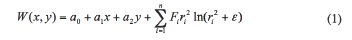
The fundamental step in this process is finding the contour line nearest to an interpolated point P and obtaining a perpendicular foot B from point P to this contour line. Then, using P–B as the base direction, eight-half lines are drawn at intervals of 45° to produce rays in eight directions. These half lines intersect with two adjacent contour lines around P, resulting in a maximum of 16 intersection points denoted by P1, P2, P3, and so on. If the number of sample points, n, is less than 16, the results will reflect the geomorphic features of the terrain adequately. Conversely, if n > 16, the efficiency of the method will be impacted negatively. Figure 5 presents an example in which 16 intersection points are obtained for the interpolated P. We use a spline function to construct an interpolation function, as described by Curry and Schoenberg (1996) and Yu (2001):

where x and y are coordinates, w (x,y) is the elevation value of interpolated point P, and α₀, α₁, α₂, and Fi (i = 1,2,...,n) are undetermined coefficients, of which there are N + 3 in total. r ²_i = (x-x_i)² + (y-y_i)² and e are empirical parameters that allow for the adjustment of surface curvature. For large (small) changes in the surface shape, ɛ should be small (large); values of e range from 10^-2 to 1 for flat surfaces and 10^-6 to 10^-5 for singularity surfaces.

The N + 3 unknowns are determined according to Equation 2.

The coefficient c^j, which is in units of length squared, is equal to 16πD/K^j, where D is the plate rigidity and K^j the spring constant associated with the j^th point. During interpolation, K^j = ∞ and c^j = 0.

2.2. Introduction of virtual control points

To ensure that the interpolated results can be constrained by the values of the contour lines, virtual control points were added to control the precision of interpolation. It was designated E_n as the value of a point on the contour line near P and E_ci as the contour interval. From the features of the contour map, it is clear that, if P is located between two contour lines, w (x,y) should lie between the values of these two contour lines. Similarly, if P is within a closed contour line, w (x,y) should be less than E_n + E_ci or larger than E_n − E_ci. If not, then this may lead to wrong results. Therefore, to prevent sudden changes from occurring in complex areas, we add a virtual control point V for the four intersection points. Then, our algorithm calculates the elevation value at point V based on the heights of the four surrounding points, according to the following rules.

The elevation of V is Z_v, which is calculated according to Equation 3.

where δ is a coefficient between 0 and 1 and is used to control the elevation of V. The adding and subtracting operations were used for DEMs covering mountaintops and depressions.

Figure 6 illustrates a typical example of the addition of a virtual control point in one direction for a case in which the interpolated point lies along an adjacent contour line. In this case, the elevation value of V should be larger than H_BC (where H_BC is the height of the contour line located using B and C) but lower than H_BC + Δh (where Δh is the interval of the contour lines). θ₁ and θ₂ denote the inclinations of lines AB and CD, respectively, and δ can be set according to the geomorphic feature studied:

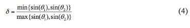
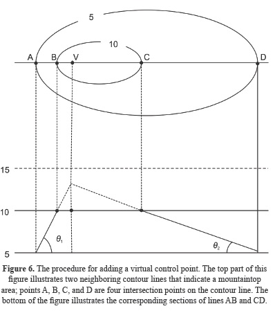
δ ranges from 0 to 1 and is equal to 1 when θ₁ = θ₂. Based on the features of the contour line map, it is clear that z_V should be less than H_BC + Δh; however, when δ = 1, z_V will be equal to H_BC + Δh. To avoid z_V reaching this value, a small perturbation (ɛ, equal to 0.01) is added to δ such that δ = 0.99. When θ₁ ≠ θ₂, δ will be greater than 0 and less than 1 and Equation 3 can be rewritten as follows:

Subsequently, the coordinates and elevation of the virtual control point can be determined. Here, E donates the intersection of lines AB and CD, and its coordinates can be obtained by solving Equations 6 and 7.

Then, the value of sin(θ₁) can be obtained as follows.

sin(θ₂) can be calculated in a similar manner. Thus, when both sin(θ₁) and sin(θ₂) are known, the elevation of the virtual control point can be obtained from Equation 3.

As discussed above, rays in eight directions are used to query the intersections with the contour lines. However, two intersection points are not present in all directions, e.g., if the interpolated point is at a boundary or corner of the map. Therefore, geomorphic information is missing in such directions. Moreover, it is not necessary to add a virtual control point in cases where there are no intersection points in a particular direction because this virtual point may introduce obvious error. If there is only one intersection point in a particular direction, two intersection points are used on the symmetrical contour lines; this produces three crossing points in total, which is sufficient to determine whether a virtual control point is required based on the geomorphic trend inferred from the three points.

There are three possible situations in cases with three points (Figure 7).

1) When the elevation of the intersection point is higher than that of either A or B (e.g., D1 in Figure 7), the geomorphic trend gets higher from A to D1, so the interpolated point is just between B and D1, and no virtual control point is required.

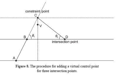
2) When the elevation of the intersection point is equal to that of A or B or lower than that of B (e.g., D2 in Figure 7), it can be assumed that the local maximum occurs at B (or in its vicinity) and that the elevation of the local maximum will never exceed HBC + Δh. A virtual control point must be added in such cases. For example, line AB could be extended to intersect the constraint contour (i.e., point C in Figure 8). Here, C acts to limit the elevation of the virtual control point. Then, the method described above can be applied to compute the coordinates and elevations of virtual points using the points A, B, C, and D.

3) When the height of the intersection is lower than that of B (e.g., D3 in Figure 7), it can be assumed that B represents the local maximum; in such cases, the geomorphic trend is clear, and no control point is required.

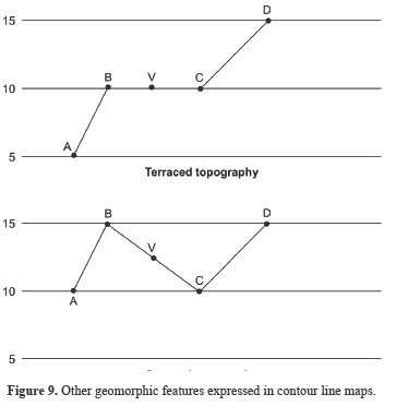
In other cases, such as where the topography is terraced or serrated (Figure 9), the elevation and location of V reflect the average of the neighboring intersection points and the midpoint of line BC, respectively. The distances between all of the virtual control points were calculated adding and removing the control point if the distance is less than a threshold value. Then, all of the remaining distances between virtual control points are above the threshold value. Different threshold values were used to test the algorithm; according to the experimental results, the threshold value should be set to 2–3 times the interpolation accuracy. Finally, it was constructed the interpolation equation using all of the virtual control points and intersection points and calculate the value of point P based on the interpolation equation.

2.3. Algorithm workflow

Here, it was introduced an efficient algorithm that achieves the interpolation of DEMs from contour maps, as shown in Figure 10. The main steps in this algorithm workflow can be summarized as follows. First, the contour lines of the map were traversed and decomposed, before dividing them into line segments and saving them. This procedure allows obtaining the average length of the line segments. Then, the R-tree indexes for these line segments were built and stored the elevation in the R-tree (Huang, P. Lin and H. Lin, 2001; Corral and Almendros-Jiménez, 2007; Zhu, Gong and Zhang, 2007). Finally, each interpolated point A was processed as follows. 1) The R-tree was used to query the closest line segment and point (i.e., B) to point A on the line segment. 2) A step K was set, whose value is equal to the average length of the line segments, and extend line AB in two directions at intervals of K. In this manner, it was assessed whether line AB intersects with the contour line, find the intersection points in both directions along line AB, and add a virtual control point if the interpolated position is on a closed contour line (Figure 11). 3) There were constructed eight lines at intervals of 45°, find the associated intersection points, and add virtual control points where appropriate. 4) It was filtered the control points according to the distance between virtual control points based on a filtering rule, which states that the distances between the added virtual control points must be above a threshold value, i.e., 2–3 times the interpolation accuracy. 5) There were calculated the coefficients of the spline interpolation function, which are determined according to the control points, and calculated the interpolated point value based on the spline interpolation feature. (6) Finally, it was output the value of the interpolated point.

3. Experiments and discussion

3.1. Experimental data and preprocessing

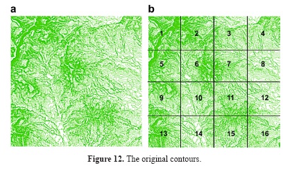
In the present study, it was validated a method using a surface contour line map for the Dayang coal mine in Shanxi Province, China. The original contour map for this area is shown in Figure 12. The original contour interval is 5 m, and the output DEM data is in the form of an ASCII grid text file with a grid cell size of 2 m. The original contour map was cut into 16 sub-maps to test the results of the proposed method (Figure 12b), and those maps were used to verify the accuracy of interpolation. Then, it was generated the DEM data for each subarea using the “Topo to Raster” function of ArcGIS, the regional interpolation method of Yu and Tan (2002), and the method proposed in this study.

3.2. Results and discussion

It was used a stretched color ramp to display the DEM results. Obvious errors (i.e., abnormal colors, indicated by red color in Figure 13) were found in the results achieved using the method of Yu and Tan (2002). However, neither the proposed method, not the ArcGIS method produce obvious errors. In fact, the results obtained using the “Topo to Raster” function of ArcGIS are very similar to the results obtained with this method; thus, they are illustrated in Figure 13.

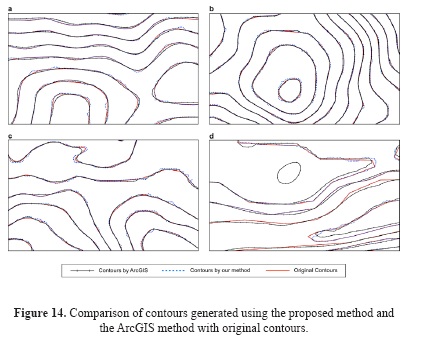
The DEM results were transformed into contour line maps to compare the results in more detail, and to set the intervals and baselines of these maps to be the same as those of the original contour map (Figure 14). It was found that, in most cases, the contour lines generated by the proposed DEM fit the original contour lines very well. Moreover, in some areas, the results agree more closely with the original contour lines than the contours generated using the ArcGIS method. In fact, the ArcGIS method is found to produce obvious errors (e.g., Figure 14d, in which a closed contour line was generated according to the ArcGIS method), suggesting that the proposed method provides more accurate DEMs that can reflect geomorphic features more closely. It was noted that the smoothing effect of the contour lines is less developed in the proposed method than in the ArcGIS's method (Figure 14). Furthermore, the proposed method generates more isolated points on the contour lines than other methods, because each DEM grid value is interpolated dynamically using intersection points and virtual control points in this approach, then smoothness is not so good.

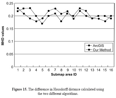
Finally, the transformed contour line maps were compared with the original map using the mean Hausdorff distance (MHD; Chen, Ma, Xu, Paul, 2010; Hung and Yang, 2004). The Hausdorff distance is a measure of the similarities between two nonempty compact (closed and bounded) sets A and B in a metric space S on their positions (Nadler, 1978). The MHD between the original and transformed contour line maps was calculated for each submap and the MHDs obtained were compared between the proposed method and the ArcGIS method (Figure 15). The results illustrate that the errors for each algorithm are similar; therefore, it was concluded that the proposed method exhibits similar accuracy to the ArcGIS process.

4. Conclusions

Here, it was presented an improved method of generating gridded DEMs from contour line maps while taking geomorphic information into account. First, it was identified the point on a contour line that is nearest to the interpolated point; the choice of this position plays a critical role in interpolation accuracy. Then, 16 points on neighboring contour lines were obtained in eight directions from the interpolated point; these points can reflect the basic geomorphic features of the resulting DEM. For regions of complex geomorphology, it was inserted a virtual control point at a specified place in each direction according to various geomorphic features identified from the original map, which prevents the interpolation result from exceeding the contour interval. Finally, the points with feature geomorphic information were used to construct local surface spline functions for interpolation. The method was tested using a surface contour line map of the Dayang coal mine in Shanxi Province, China, and the results were compared with those obtained using existing methods. It was concluded that the proposed method is at least as accurate as the ArcGIS “Topo to Raster” function and is more accurate than the method described by Yu and Tan (2002).

In this method, each DEM grid value is interpolated based on intersection points and virtual control points, and the spline interpolation function was constructed dynamically. Therefore, the method requires a greater analysis time than the ArcGIS method and the DEMs generated using it are not as smooth as those generated using the ArcGIS method. Improvements in this regard will form the basis of future work. The interpretation of real complex geomorphic features from contour maps remains challenging, and the objective of this study is to continue improving the methods for interpolation of gridded DEM data based on such maps.

Funding

This work was supported by the National Science and Technology Major Project of China [No. 2011ZX05039-004], the National Natural Science Foundation of China [No. 40901191], the Strategic Priority Research Program of the Chinese Academy of Sciences [No. XDA05030200], the Hebei Province Natural Science Fund [No. D2016210008], the Social Science Foundation Project of Hebei Province [No. HB15SH015], and the Scientific Research Foundation for Doctor of Shijiazhuang Tiedao University.

---

References.

Aumann, G., Ebner, H. & Tang, L. (1991). Automatic derivation of skeleton lines from digitized contours. ISPRS Journal of Photogrammetry and Remote Sensing, 46, 259-268. DOI: 10.1016/0924-2716(91)90043-U.

Binh, T. Q. and Thuy, N. T. (2008). Assessment of the influence of interpolation techniques on the accuracy of digital elevation model. VNU Journal of Science, Earth Sciences, 24(4), 176-183.

Bonin, O., & Rousseaux, F. (2005). Digital Terrain Model Computation from Contour Lines: How to Derive Quality Information from Artifact Analysis. Geoinformatica, 9(3), 253-268. DOI: 10.1007/s10707-005-1284-2.

Bouillon, A., Bernard, M., Gigord, P., Orsoni, A., Rudowski, V., and Baudoin, A. (2006). SPOT 5 HRS geometric performances: Using block adjustment as a key issue to improve quality of DEM generation. ISPRS Journal of Photogrammetry and Remote Sensing, 60(3), 134-146. DOI: 10.1016/j.isprsjprs.2006.03.002.

Carley, J. K., Pasternack, G. B., Wyrick, J. R., Barker, J. R., Bratovich, P. M., Massa D. A., ... Johnson T. R. (2012). Significant decadal channel change 58-67 years post-dam accounting for uncertainty in topographic change detection between contour maps and point cloud models. Geomorphology, 179, 71-88. DOI: 10.1016/j.geomorph.2012.08.001.

Carrara, A., Bitelli, G., & Carla, R. (1997). Comparison of techniques for generating digital terrain models from contour lines. International Journal of Geographical Information Science, 11(5), 451-473.

Chen, X., Ma, W., Xu, G., & Paul, J. C. (2010). Computing the Hausdorff distance between two B-spline curves. Computer-Aided Design, 42(12), 1197-1206. DOI: 10.1016/j.cad.2010.06.009.

Clarke, A. L., Gruen, A., & Loon, J. C. (1982). The application of contour data for generating high fidelity grid digital elevation models. Proceedings Auto-Carto 5, 213-222. Washington DC.

Corral, A., & Almendros-Jiménez, J. M. (2007). A performance comparison of distance-based query algorithms using R-trees in spatial databases. Information Sciences, 177(11), 2207-2237. DOI: 10.1016/j.ins.2006.12.012.

Curry, H. B., & Schoenberg, I. J. (1996). On Pólya frequency functions IV: The fundamental spline function and their limits. Journal d'Analyse Mathematique, 17(1), 71-107. DOI: 10.1007/BF02788653.

Dinis, L. M. J. S., Natal Jorge, R. M., & Belinha, J. (2007). Analysis of 3D solids using the natural neighbour radial point interpolation method. Computer Methods in Applied Mechanics and Engineering, 196(13-16), 2009-2028. DOI: 10.1016/j.cma.2006.11.002.

Doytsher, Y., & Hall J. K. (1997). Interpolation of DTM using bi-directional third-degree parabolic equations, with FORTRAN subroutines. Computers & Geosciences, 23(9), 1013-1020. DOI: 10.1016/S0098-3004(97)00061-7.

Gofuku, S., Tamura, S., & Maekawa, T. (2009). Point-tangent/point-normal B-spline curve interpolation by geometric algorithms. Computer-Aided Design, 41(6), 412-422. DOI: 10.1016/j.cad.2009.02.005.

Gousie, M. B., & Franklin W. R. (2003). Constructing a DEM from grid-based data by computing intermediate contours. In GIS 2003: Proceedings of the Eleventh ACM International Symposium on Advances in Geographic Information Systems, 71-77. DOI: 10.1145/956676.956686.

Hearnshaw, H. M., & Unwin, D. J. (1994). Visualization in Geographical Information Systems. Chichester: Wiley, 168-180.

Heritage, G. L., Milan, D. J., Large, A. R. G., & Fuller, L. C. (2009). Influence of survey strategy and interpolation model on DEM quality. Geomorphology, 112(3-4), 334-344. DOI: 10.1016/j.geomorph.2009.06.024.

Hickey, R., Smith A., & Jankowski P. (1994). Slope length calculations from a DEM within ARC/INFO grid. Computers, Environment and Urban Systems, 18(5), 365-380. DOI: 10.1016/0198-9715(94)90017-5.

Huang, F., Liu, D., Tan, X., Wang, J., Chen Y., & He, B. (2011). Explorations of the implementation of a parallel IDW interpolation algorithm in a Linux cluster-based parallel GIS. Computers & Geosciences, 37(4), 426-434. DOI: 10.1016/j.cageo.2010.05.024.

Huang, P. W., Lin, P. L., & Lin, H. Y. (2001). Optimizing storage utilization in R-tree dynamic index structure for spatial databases. Journal of Systems and Software, 55(3), 291-299. DOI: 10.1016/S0164-1212(00)00078-9.

Hung, W., & Yang, M. (2004). Similarity measures of intuitionistic fuzzy sets based on Hausdorff distance. Pattern Recognition Letters, 25(14), 1603-1611. DOI: 10.1016/j.patrec.2004.06.006.

Hutchinson, M. F. (1988). Calculation of hydrologically sound digital elevation models. Third International Symposium on Spatial Data Handling, Sydney, Australia, August 117-133.

Hutchinson, M. F. (1996). A locally adaptive approach to the interpolation of digital elevation models. In Proceedings, Third International Conference/Workshop on Integrating GIS and Environmental Modeling, January 21-25.

Hutchinson, M. F. (2008). Adding the Z-dimension. In Wilson J.P. and Fotheringham, A. S. (Eds.) The Handbook of Geographic Information Science, (pp. 144-168). Blackwell. DOI: 10.1002/9780470690819.ch8.

Jones, K. H. (1998). A comparison of algorithms used to compute hill slope as a property of the DEM. Computers & Geosciences, 24(4), 315-323. DOI: 10.1016/S0098-3004(98)00032-6.

Kweon, I. S. and Kanade T. (1994). Extracting Topographic Terrain Features from Elevation Maps. CVGIP: Image Understanding, 59(2), 171-182.

Li, Z. (1994). A comparative study of the accuracy of digital terrain models (DTMs) based on various data models. ISPRS Journal of Photogrammetry and Remote Sensing, 49(1), 2-11.

Maekawa, T., Matsumoto, Y., & Namiki, K. (2007). Interpolation by geometric algorithm. Computer-Aided Design, 39(4), 313-323. DOI: 10.1016/j.cad.2006.12.008.

Nadler, S. B. (1978). Hyperspaces of sets: A text with research questions. New York: Marcel Dekker.

Oky, P., Ardiansyah, D., & Yokoyama R. (2002). DEM generation method from contour lines based on the steepest slope segment chain and a monotone interpolation function. ISPRS Journal of Photogrammetry and Remote Sensing, 57(1-2), 86-101. DOI: 10.1016/S0924-2716(02)00117-X.

Peralvo, M., and Maidment, D. (2008). Influence of DEM Interpolation Method in Drainage Analysis. Available online at www.crwr.utexas.edu/gis/gishydro04/Introduction/TermProjects/Peralvo.pdf.

Rvachev, V. L., Sheiko, T. I., Shapiro, V., & Tsukanov, I. (2001). Transfinite interpolation over implicitly defined sets. Computer Aided Geometric Design, 18(3), 195-220. DOI: 10.1016/S0167-8396(01)00015-2.

Taud, H., Parrot, J. F., & Alvarez, R. (1999). DEM generation by contour line dilation. Computers & Geosciences, 25(7), 775-783. DOI: 10.1016/S0098-3004(99)00019-9.

Vieux, B. E. (1993). DEM aggregation and smoothing effects on surface runoff modeling. Journal of Computing in Civil Engineering-ASCE, 7(3), 310-338. DOI: 10.1061/(ASCE)0887-3801(1993)7:3(310).

Wang, D., Tian, Y., Gao Y., & Wu. L. (2005). A New Method of Generating Grid DEM from Contour Lines. IGARSS 2005, 657-660. DOI: 10.1109/IGARSS.2005.1526261.

Watson, D. F. (1992). Contouring: A Guide to the Analysis and Display of Spatial Data. Oxford: Pergamon.

Watson, D. (1999). The natural neighbor series manuals and source codes. Computers & Geosciences, 25(4), 463-466. DOI: 10.1016/S0098-3004(98)00150-2.

Werbrouck, I., Antrop, M., Van Eetvelde, V., Stal, C., De Maeyer, P., Bats, M., ... Zwertvaegher, A. (2011). Digital elevation model generation for historical landscape analysis based on LiDAR data, a case study in Flanders (Belgium). Expert Systems with Applications, 38(7), 8178-8185. DOI: 10.1016/j.eswa.2010.12.162.

Wise, S. (2011). Cross-validation as a means of investigating DEM interpolation error. Computers & Geosciences, 37(8), 978-991.

Wise, S. (2012). Information entropy as a measure of DEM quality. Computers & Geosciences, 48, 102-110. DOI: 10.1016/j.cageo.2012.05.011.

Wood, J. (1994). Visualizing contour interpolation accuracy in digital elevation models. In H. M. Hearnshaw and D. J. Unwin, eds. Visualization in geographical information systems. Chichester: John Wiley and Sons, 168-180.

Wood, J. D., & Fisher P. F. (1993). Assessing interpolation accuracy in elevation models. IEEE Computer Graphics and Applications, 13(2), 48-56. DOI: 10.1109/38.204967.

Xiao, L., & Liu, H. (2012). A novel approach for quantitative assessment of DEM accuracy using reconstructed contours. Procedia Environmental Sciences, 12 Part B, 772-776. DOI: 10.1016/j.proenv.2012.01.346.

Xie, K., Wu, Y., Ma, X., Liu, Y., Liu, B., & Hessel, R. (2003). Using contour lines to generate digital elevation models for steep slope areas: a case study of the Loess Plateau in North China. Catena, 54(1-2), 161-171. DOI: 10.1016/S0341-8162(03)00063-8.

Yu, Z. W. (2001). Surface interpolation from irregularly distributed points using surface splines, with Fortran program. Computers & Geosciences, 27(3), 877-882.

Yu, Z. W., & Tan, H. Q. (2002). Regionalized interpolation: A new approach to surface map reconstruction. Terra Nostra, 3, 513-517.

Zhou, Q., & Chen Y. (2011). Generalization of DEM for terrain analysis using a compound method. ISPRS Journal of Photogrammetry and Remote Sensing, 66(1), 38-45. DOI: 10.1016/j.isprsjprs.2010.08.005.

Zhou, Q., & Liu X., (2004). Analysis of errors of derived slope and aspect related to DEM data properties. Computers & Geosciences, 30(4), 369-378. DOI: 10.1016/j.cageo.2003.07.005.

Zhu, Q., Gong, J., & Zhang, Y. (2007). An efficient 3D R-tree spatial index method for virtual geographic environments. ISPRS Journal of Photogrammetry and Remote Sensing, 62(3), 217-224. DOI: 10.1016/j.isprsjprs.2007.05.007.