Shear-wave velocity structure of Australia from Rayleigh-wave analysis

The elastic structure beneath Australia is shown by means of S-velocity maps for depths ranging from zero to 400 km, determined by the regionalization and inversion of Rayleigh-wave dispersion. The traces of 233 earthquakes, occurred from 1990 to 2010, have been used to obtain Rayleigh-wave dispersion data. These earthquakes were registered by 65 seismic station located in Australia and the surrounding area. The dispersion curves were obtained for periods between 5 and 250 s, by digital filtering with a combination of MFT (Multiple Filter Technique) and TVF (Time Variable Filtering), filtering techniques. Later, all seismic events (and some stations) were grouped to obtain a dispersion curve for each source-station path. These dispersion curves were regionalized and inverted according to the generalized inversion theory, to obtain shear-wave velocity models for a rectangular grid of 2.5°×2.5° mesh size. The shear-velocity structure obtained through this procedure is shown in the S-velocity maps plotted for several depths. These results agree well with the geology and other geophysical results previously obtained. The obtained S-velocity models suggest the existence of lateral and vertical heterogeneity. The zones with consolidated and old structures present greater S-velocity values than those in the other zones, although this difference can be very little or negligible in some case. Nevertheless, in the depth range of 15 to 50 km, the different Moho depths present in the study area generate the principal variation of S-velocity. A similar behaviour is found for the depth range from 65 to 180 km, in which the lithosphere-asthenosphere boundary generates the principal variations of S-velocity. Finally, it should be highlighted a new and interesting feature was obtained in this study: the definition of the base of the asthenosphere, for depths ranging from 155 to 280 km, in Australia and the surrounding area. This feature is also present in the continents: South America, Antarctica and Africa, which were part of the same super-continent Gondwanaland, in the early Mesozoic before fragmentation.

La estructura elástica bajo Australia es mostrada por medio de mapas de velocidad de onda S, para profundidades que varían desde cero a 400 km, determinada por regionalización e inversión de dispersión de ondas Rayleigh. Las trazas de 233 terremotos, ocurridos desde 1990 hasta 2010, han sido usadas para obtener datos de dispersión de ondas Rayleigh. Estos terremotos fueron registrados por 65 estaciones sísmicas localizadas en Australia y el área circundante. Las curvas de dispersión fueron obtenidas para periodos entre 5 y 250 s, por filtrado digital con una combinación de las técnicas de filtrado: MFT (técnica del filtro múltiple) y TVF (filtrado en tiempo variable). Luego, todos los eventos sísmicos (y algunas estaciones) fueron agrupados para obtener una curva de dispersión para cada trayecto fuente-estación. Estas curvas de dispersión fueron regionalizadas e invertidas de acuerdo con la teoría de la inversión generalizada, para obtener modelos de velocidad de onda de cizalla para una rejilla regular de tamaño de celda de 2.5°×2.5°. La estructura de velocidad de cizalla obtenida a través de este procedimiento es mostrada en los mapas de velocidad de onda S representados para diversas profundidades. Estos resultados concuerdan bien con la geología y otros resultados geológicos y geofísicos previamente obtenidos. Los modelos de velocidad de onda S obtenidos sugieren la existencia de heterogeneidad lateral y vertical. Las zonas con estructuras antiguas y bien consolidadas presentan mayores valores de velocidad de onda S que los correspondientes a otras zonas, aunque esta diferencia puede ser muy pequeña o despreciable en algún caso. No obstante, en el rango de profundidad de 15 a 50 km, las diferentes profundidades del Moho presentes en el área de estudio generan la principal variación de velocidad de onda S. Un comportamiento similar es encontrado par el rango de profundidad desde 65 a 180 km, en el cual la frontera litosfera-astenosfera genera la principal variación de velocidad de onda S. Finalmente, debería ser notado que una nueva e interesante característica fue obtenida en este estudio: la definición de la base de la astenosfera, para profundidades que varían desde 155 a 280 km, en Australia y el área circundante. Esta característica está también presente en los continentes: América del Sur, Antártida y África, los cuales fueron parte del mismo súper-continente: Gondwana, en el Mesozoico temprano antes de fragmentarse.

https://doi.org/10.15446/esrj.v18n2.41078

V. Corchete¹

¹ Higher Polytechnic School, University of Almeria. Almeira. España
email: corchete@ual.es

Record:
Manuscript received: 05/12/2013 Accepted for publication: 21/09/2014

---

ABSTRACT

The elastic structure beneath Australia is shown by means of S-velocity maps for depths ranging from zero to 400 km, determined by the regionalization and inversion of Rayleigh-wave dispersion. The traces of 233 earthquakes, occurred from 1990 to 2010, have been used to obtain Rayleigh-wave dispersion data. These earthquakes were registered by 65 seismic station located in Australia and the surrounding area. The dispersion curves were obtained for periods between 5 and 250 s, by digital filtering with a combination of MFT (Multiple Filter Technique) and TVF (Time Variable Filtering), filtering techniques. Later, all seismic events (and some stations) were grouped to obtain a dispersion curve for each source-station path. These dispersion curves were regionalized and inverted according to the generalized inversion theory, to obtain shear-wave velocity models for a rectangular grid of 2.5°×2.5° mesh size. The shear-velocity structure obtained through this procedure is shown in the S-velocity maps plotted for several depths. These results agree well with the geology and other geophysical results previously obtained. The obtained S-velocity models suggest the existence of lateral and vertical heterogeneity. The zones with consolidated and old structures present greater S-velocity values than those in the other zones, although this difference can be very little or negligible in some case. Nevertheless, in the depth range of 15 to 50 km, the different Moho depths present in the study area generate the principal variation of S-velocity. A similar behaviour is found for the depth range from 65 to 180 km, in which the lithosphere-asthenosphere boundary generates the principal variations of S-velocity. Finally, it should be highlighted a new and interesting feature was obtained in this study: the definition of the base of the asthenosphere, for depths ranging from 155 to 280 km, in Australia and the surrounding area. This feature is also present in the continents: South America, Antarctica and Africa, which were part of the same super-continent Gondwanaland, in the early Mesozoic before fragmentation.

Key Words: Rayleigh wave, Shear wave, crust, upper mantle, Australia.

---

RESUMEN

La estructura elástica bajo Australia es mostrada por medio de mapas de velocidad de onda S, para profundidades que varían desde cero a 400 km, determinada por regionalización e inversión de dispersión de ondas Rayleigh. Las trazas de 233 terremotos, ocurridos desde 1990 hasta 2010, han sido usadas para obtener datos de dispersión de ondas Rayleigh. Estos terremotos fueron registrados por 65 estaciones sísmicas localizadas en Australia y el área circundante. Las curvas de dispersión fueron obtenidas para periodos entre 5 y 250 s, por filtrado digital con una combinación de las técnicas de filtrado: MFT (técnica del filtro múltiple) y TVF (filtrado en tiempo variable). Luego, todos los eventos sísmicos (y algunas estaciones) fueron agrupados para obtener una curva de dispersión para cada trayecto fuente-estación. Estas curvas de dispersión fueron regionalizadas e invertidas de acuerdo con la teoría de la inversión generalizada, para obtener modelos de velocidad de onda de cizalla para una rejilla regular de tamaño de celda de 2.5°×2.5°. La estructura de velocidad de cizalla obtenida a través de este procedimiento es mostrada en los mapas de velocidad de onda S representados para diversas profundidades. Estos resultados concuerdan bien con la geología y otros resultados geológicos y geofísicos previamente obtenidos. Los modelos de velocidad de onda S obtenidos sugieren la existencia de heterogeneidad lateral y vertical. Las zonas con estructuras antiguas y bien consolidadas presentan mayores valores de velocidad de onda S que los correspondientes a otras zonas, aunque esta diferencia puede ser muy pequeña o despreciable en algún caso. No obstante, en el rango de profundidad de 15 a 50 km, las diferentes profundidades del Moho presentes en el área de estudio generan la principal variación de velocidad de onda S. Un comportamiento similar es encontrado par el rango de profundidad desde 65 a 180 km, en el cual la frontera litosfera-astenosfera genera la principal variación de velocidad de onda S. Finalmente, debería ser notado que una nueva e interesante característica fue obtenida en este estudio: la definición de la base de la astenosfera, para profundidades que varían desde 155 a 280 km, en Australia y el área circundante. Esta característica está también presente en los continentes: América del Sur, Antártida y África, los cuales fueron parte del mismo súper-continente: Gondwana, en el Mesozoico temprano antes de fragmentarse.

Palabras clave: Estructura de velocidad de onda S de Australia a partir del análisis de ondas Rayleigh.

---

1. Introduction

The great ability of the Rayleigh-wave dispersion analysis to delineate the Earth's deep structure is well known (Corchete, 2012). This methodology allows the features of the Earth's structure to be determined, because it is well known that the surface-wave dispersion (Rayleigh-wave dispersion) is related to the Earth's structure crossed by the waves (represented by the S-velocity structure). Thus, the features of the elastic structure for any region of Earth can be studied through the analysis of Rayleigh-wave dispersion. In this paper, the features of the elastic structure beneath Australia (and the surrounding area) will be revealed through this analysis. Australia and its surrounding area are ones of the regions for which there are relatively few seismic studies concerning deep mantle structure (e.g. Zielhuis and van der Hilst, 1996; Simons et al. 1999; Fichtner et al., 2009; Fishwick and Rawlinson, 2012). Since the geologic setting of this area is very complex, knowledge of detailed seismic structure of this area would be of great importance. Nevertheless, the elastic structure beneath Australia is among the least studied structures on Earth, due to the particular conditions of this continent (a large part is covered by deserts), which have made difficult the development and maintenance of high-quality seismic networks. Fortunately, in the recent years, some international agencies (as GSN, IRIS GEOFON and GEOSCOPE) joint to local agencies (as Geoscience Australia) have been able to develop and support new and permanent broad-band digital seismic stations (and portable deployments within Australia). As a result, in the last twenty years high-quality seismic records have been made available from seismographic databases for Australia and its surrounding area.

In pioneer studies, Ellis and Denham (1985) and Denham and Ellis (1986) investigated the crust and upper mantle structure using surface waves. They used periods of the fundamental modes ranged from 8 to 60 s, obtaining a few shear-velocity profiles from 0 to 140 km of depth. Later, Zielhuis and van der Hilst (1996) performed the first Rayleigh-wave tomography for Australia and the surrounding area. In this study, they constructed a 3-D model of shear velocity for the upper mantle (and transition zone beneath eastern Australia and the adjacent oceanic regions), using both body and Rayleigh waves (fundamental and higher modes). They obtained shear-velocity maps from 80 to 400 km of depth (although the resolution decreases drastically with depth from 200 km). Few years later, Simons et al. (1999) performed a more complete Rayleigh-wave tomography for Australia and the surrounding area. In this study, they obtained shear velocity maps from 80 to 400 km of depth (although the resolution decreases drastically with depth from 210 km), using periods of fundamental modes ranged from 40 to 200 s and periods of higher modes ranged from 20 to 125 s. More recently, Fishwick et al. (2005), Fishwick and Reading (2008) and Fishwick and Rawlinson (2012) obtained the upper-mantle S-velocity structure beneath Australia, from surface-wave tomography, for depths ranging from 75 to 300 km (although the resolution decreases drastically with depth from 225 km). Fishwick and Rawlinson (2012) compared their surface-wave inversion results with those calculated by Fishwick et al. (2008), finding very similar patterns of S-velocity in both studies (also in both studies the resolution decreases drastically with depth from 225 km). The results obtained by Fishwick and Rawlinson (2012) are also very similar to those calculated by Fichtner et al. (2009), who obtained the upper-mantle S-velocity structure in the Australasian region, from a full seismic waveform tomography, for depths ranging from 80 to 400 km (although the resolution of their 3D S-velocity model decreases drastically with depth from 250 km). Finally, Saygin and Kennett (2012) obtained the first 3-D S-velocity structure for the Australian crust (from 0 to 30 km of depth), using surface-wave group velocity (from 1 to 32 s of period) extracted from ambient noise. This S-velocity model for the crust was combined with all the information retrieved from the above-mentioned studies, by Kennett and Salmon (2012), to perform their AuSREM (Australian Seismological Reference Model). This recent model is displayed from 0 to 400 km of depth (although its resolution decreases drastically with depth from 225 km). In the crust, AuSREM represents the Australian crust via a 5-layered structure (i. e. only 5 layers are considered for the whole Australian crust). These five layers are: sediments, basement, upper crust, middle crust and lower crust. This simple form to give a model for the crust, provides considerable flexibility to be used in seismic-receiver function studies, but it provides considerable lesser information than the S-velocity model performed by Saygin and Kennett (2012), which is a true 3D model (although it is only displayed from 0 to 30 km of depth).

It should be noted that no 3D S-velocity structure has been obtained for Australia and its surrounding area, from surface-wave tomography, for depths ranging from 30 to 75 km. Furthermore, the S-velocity structure, obtained in the above-mentioned previous studies, shows a poor resolution for the depth range from 200 to 400 km. For it, the goal of the present study is the determination of the elastic structure (S-velocity structure) beneath Australia and the surrounding area, from Rayleigh-wave analysis, for the whole depth range from 0 to 400 km, because no 3D S-velocity structure has been obtained, until now, for this study area in this complete depth range. This Rayleigh-wave analysis will consist of filtering of Rayleigh waves, to obtain dispersion curves from 5 to 250 s. This dispersion analysis will be performed in several steps. First, all seismic events will be grouped in source zones to get an average dispersion curve for each source-station path. Then, the dispersion curves will be obtained by digital filtering with a combination of the Multiple Filter Technique (Dziewonski et al., 1969) and Time Variable Filtering (Cara, 1973). Thus, a set of source-station averaged dispersion curves will be calculated. This set of dispersion curves will be regionalized and then inverted according to the generalized inversion theory, to get S-wave velocity models for a rectangular grid defined in the study area. Finally, these models will be plotted to obtain a 2D mapping of the 3D S-wave velocity structure, for the study area. The period range to be obtained in the present study, by digital filtering, will be wider than the period range measured in the above-mentioned previous studies. Thus, the determination of the 3D S-velocity structure, in the whole depth range from 0 to 400 km, will be more accurate in the present study than the other above-mentioned previous studies, in which no surface-wave dispersion was measured in the period ranges from 5 to 40 s and from 200 to 250 s. This lack of information in the above-mentioned previous studies has caused the lack of a 3D S-velocity structure, for the depth range from 0 to 80 km, and the bad resolution of the 3D S-velocity structure for the depth range from 200 to 400 km.

2. Data set

In this study, a list of 233 earthquakes, occurred from 1990 to 2010 in the neighbouring of Australia, was considered (Supplement 1). These earthquakes were registered by 65 seismic stations located at this continent and the surrounding area (Supplement 2). From these stations digital data are available, recorded with a different instrument for each available channel (Supplement 6). From all these channels, only the records for the channels: BHZ, LHZ, BLZ, LLZ, BH1, LH1, BH2, LH2; have been considered as the most suitable data for this study, because the period interval of the best registration for these channels is between 1 or 5 to 200 or 250 s (period interval in which the frequency response is almost flat). This period interval (from 1 to 250 s) is more suitable for exploring the elastic structure of the Earth, for a depth range of 0 to 400 km of depth. For this reason, the above mentioned channels haven been selected from the all available channels.

Also, to ensure the reliability of the results, only the earthquake traces in which a well-developed Rayleigh wave train is present, with a very clear dispersion, have been considered. Thus, many records have been discarded.

Logically, the instrumental response must be taken into account to avoid the time lag introduced by the seismograph system (and all distortions produced by the instrument). This correction recovers the true amplitude and phase of the ground motion, allowing the analysis of the true dispersion of Rayleigh waves. For this reason, all the traces considered in this study were corrected for instrument response.

3. Pre-processing and filtering

For the pre-processing and calculation of dispersion curves, the computation method detailed by Corchete et al. (2007) was followed. In this paper, only a brief review of the principal concepts of this methodology will be presented.

Grouping of stations and seismic events. It is well known that generally the Rayleigh waves propagated along very near epicentre-station paths show similar dispersion curves, because they cross the same earth structure and sample the same elastic properties of the medium. As a result, it is possible to group all seismic events listed in Supplement 1 in source zones, as listed in Supplement 3, to get source-station paths from epicentre-station paths. These source zones are defined as a location at which seismic events with similar epicentre coordinates have occurred. The coordinate differences for a group of events must be less than or equal to 1 degree in latitude and longitude, to be able to group them in the same source zone. Then, an average dispersion curve for each source-station path can be obtained, when the dispersion curves calculated for the traces of the events of this source zone (recorded at the same station) are averaged. In this way, any small deviations obtained are considered errors, which can be described by the standard deviation. It should be noted that some stations considered in this study also show very similar coordinates. Thus, they have been grouped using the same criteria described above for the events, defining new station codes to denote these average stations. These new stations are listed in Supplement 4. Figure 1 shows the path coverage obtained for the study area given by the source-station paths (the source coordinates are listed in Supplement 3 and the station coordinates are listed in Supplement 2 and 4).

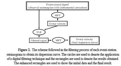
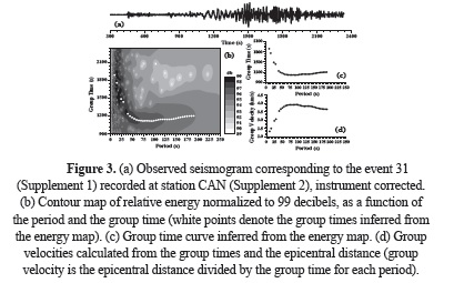
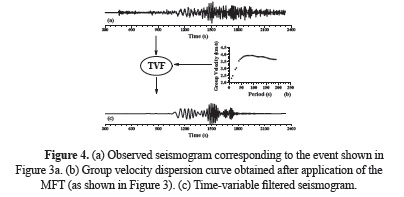
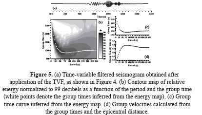
Dispersion analysis. The Rayleigh-wave group velocity for the trace of each event registered has been measured by means of the combination of digital filtering techniques: Multiple Filter Technique (MFT) and Time Variable Filtering (TVF), as shown in the flow chart displayed in Figure 2. As an example of this filtering process, the application of this combination of filtering techniques to the trace of the event 31 (recorded at station CAN) will be detailed. The MFT has been applied firstly to this trace as it is shown in Figure 3. This trace and the dispersion curve obtained are used to compute the digital filtered signal using the TVF. Figure 4 shows the time-variable filtered signal resulting from the TVF. Finally, Figure 5 shows the final dispersion curve obtained after application of the MFT to the filtered signal. A comparison between Figures 3 and 5 shows the benefits of the proposed filtering process. It should be noted that a combination of MFT and TVF works better than the application of the MFT only, because the signal/noise ratio is highly increased.

Average dispersion curves and estimation of the error. When the dispersion curves of the traces for each event involved in a source-station path have been calculated, by means of the above-described filtering process, the average group velocity for this path can be obtained as a mean of the group-velocity values calculated for each period. An estimation of the error for this media is calculated by the standard deviation (1-s error). For paths with only one event involved, a mean of the standard deviations obtained for the other near paths (which have more than one event involved), can be considered as a good estimation of the error. The average group velocities obtained for the 412 source-station paths considered in this study are listed in Supplement 5 for several periods. The periods for these dispersion curves ranges from 5 to 250 s. It should be noted that the period range obtained in the present study largely exceeds the period range obtained in previous studies (Simons et al., 1999; Fishwick et al., 2005; Fishwick and Reading, 2008; Fichtner et al., 2009). This fact points to a better determination of the elastic structure beneath Australia for large depths, if the present dispersion data are used.

4. Regionalization of group velocities

The above-described group velocities constitute the dispersion curves to be considered for regionalization. The period range of these curves goes from 5 to 250 s (Supplement 5) and there are 412 dispersion curves corresponding to the source-station paths shown in Figure 1, a dispersion curve for each source-station path. Thus, for each above-mentioned path, the forward problem in the regionalization of the surface-wave velocities is expressed as (Keilis-Borok, 1989)

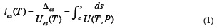
where Ues(T) is the group velocity (dispersion curve) observed between the source and the station along a great-circle path connecting those two points (the source-station path), Des is the source-station distance (Des = òds) and U(T, P) is the local group velocity at a period T and a point P of the earth surface (on the great-circle path). The inverse problem is posed to calculate the local group velocity U(T, P), at each period T and at each point P, from the average group velocity Ues(T) previously measured for a number M of source-station paths. The inverse problem defined in these terms is known as regionalization of the surface-wave velocities. This inverse problem can be simplified, if the reciprocal of the local group velocity U(T, P), or equivalently the slowness S(λ, Φ), is expanded into Fourier series by the formula

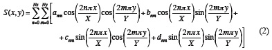
where x is λ - l₀ and y is Φ - f₀, (l₀, f₀) are the geographical longitude and latitude of the point at the bottom left corner of the study area (Figure 1), X is l_max - l₀ and Y is f_max - f₀, (l_max, f_max) are the geographical longitude and latitude of the point at the top right corner of the study area (Figure 1) and (a_nm, b_nm, c_nm, d_nm, Ny and Nx) are constants. It should be noted that U(x, y) takes the velocity values of U(T, P), i. e., U(x, y) = U(l, Φ) and S(x, y) = S(λ, Φ), for each period T, because each point P (on the earth surface considered as a sphere) has coordinates (x, y) and (λ, Φ). If formula (2) is introduced in the relationship (1) the group time can be expressed as

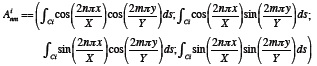
where t_i is the group time of the ith source-station path (with i =1, 2, …, M), C_i is the great-circle that connects the source and station points of the ith source-station path. M is the number of source-stations paths measured for the period T (the maximum is 412 for this study). Equations (3) also can be written in the form

where B_nm is (a_nm; b_nm; c_nm; d_nm) and

Then, equations (3) can be expressed as a system of linear equations, for each period T, in the form

Formula (4) is a set of M linear equations, for a given period T, with N unknowns x_j (with j =1, 2, …, N), where N = 4(Nx+1)(Ny+1). There is a forward problem posed for each period T, for which the equations (4) can be written. In each forward problem, the number of equations M can take different values depending on the considered period T, because the path coverage can be different for each period (Supplement 5). As a consequence of this, the number of unknowns N that can be properly determined may be also different in each problem, because always N must be less than or equals to M. Otherwise, formula (4) will be a set of equations with more unknowns N than equations M, being very difficult or impossible to determine of the unknowns x_j or equivalently the B_nm coefficients of formula (2).

Once the forward problem has been defined by formula (4), for each period T, the regionalization of the surface-wave velocities is performed by the inversion of formula (4), or equivalently inverting the matrix A. The inverse matrix of A can be obtained using the inverse method detailed by Corchete and Chourak (2010). This inverse matrix is given by

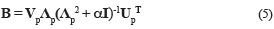
The matrix B defined by formula (5) is called the damped generalized inverse. Then, the linear equations given by formula (4) are inverted to obtain x by means of

The product of matrixes B and A is called resolution matrix and it is obtained through

If the resolution matrix given by formula (7) is the identity matrix, the obtained solution is unique and the resolution is perfect. Nevertheless, the addition of the factor a in the main diagonal makes that the equality BA = I is only reached when the damping factor a is zero. The introduction of the damping parameter degrades resolution, but stabilizes the obtained solution by means of the reduction of the variance (Corchete and Chourak, 2010). The error in the model parameters (or equivalently the error in the solution ) due to the error Dy in the data (i. e. the error in the group times), is given by the corresponding covariance matrix as (Aki and Richards, 1980)

where indicates averaging, B is given by (5) and the covariance matrix for is calculated from the covariance matrix of the error in data . Assuming that all the components of the data vector Δy are statistically independent (or assuming an independent error for each individual measurement), i. e. assuming that the fluctuation in any data is entirely independent of the fluctuation of other data, the off diagonal elements are made zero. 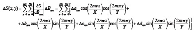Then, the main diagonal elements of the data covariance matrix are the variances of the data. If a similar behaviour is assumed for the model parameters x (i. e. assuming that all the components of the vector x are statistically independent), the off diagonal elements are made zero. Then, the main diagonal elements of the model covariance matrix are the variances of the model parameters. The obtained solution (or equivalently the set of coefficients B_nm) is calculated by introducing the relation (5) in the equations (6). Then, the slowness S(x, y), or equivalently the reciprocal U(x, y), is computed from these coefficients B_nm using formula (2). The errors in the model parameters (or equivalently the errors in the coefficients B_nm) are obtained by means of the relation (8). Later, the error in the slowness S(x, y) is computed from the errors in the coefficients B_nm using the partial derivative of formula (2) given by

Finally, the error in the local group velocity U(x, y) is computed from the error in the slowness S(x, y), using also the partial derivative of the formula

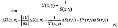
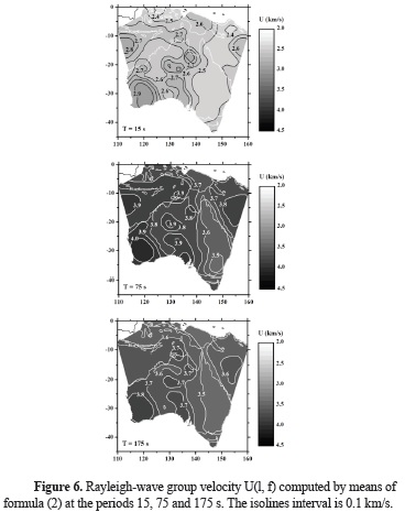
Figure 6 shows the regionalized group velocity U(λ, Φ) obtained following the above-described method for the periods 15, 75 and 175 s. Figure 7 shows the errors of the regionalized group velocity DU(λ, Φ) for the same periods. The geographical distribution of group velocities shown in Figure 6, presents the highest values for the consolidated and old structures. The group velocity presents the highest values at the western part of the continent, while the group velocity values at the eastern part are the lowest ones. This group velocity pattern agrees well with that shown in the group velocity maps performed by Saygin and Kennet (2012). Nevertheless, the group velocity maps shown in Figure 6, present a better resolution than that achieved in the group velocity mapping of Saygin and Kennet (2012). The identification of the principal geological units of Australia, in terms of group velocity, is clearer in the present study.

5. Inversion of regionalized dispersion curves

The above-described group velocity distributions with period must be inverted to obtain the shear-wave velocity distribution with depth (the 3D S-velocity structure for Australia and its surrounding area). For it, these group velocity surfaces U(λ, Φ) calculated for each period, from 5 to 250 s, are sampled in a rectangular grid with 2.5°×2.5° mesh size, from 110 to 160°E and from 0 to 45°S. These grid data can be inverted to obtain a shear velocity model (a shear velocity distribution with depth) for each grid point of the study area, achieving thus a 3D S-velocity model that represents the 3D elastic structure beneath Australia and its surrounding area, obtained from 110 to 160°E and from 0 to 45°S. The inversion of the group velocity, for each grid point of the study area, will be performed using the computation method described in detail by Corchete et al. (2007). Here only a brief review of the principal concepts of this methodology is presented.

Selection of an initial earth model. The selection of an initial earth model is a preceding step before the inversion process. The initial model must be prepared considering all information available for the study area, with respect to the S-wave, P-wave and density distributions with depth. For the present study, this geophysical and geological information has been obtained from previous studies developed in the study area, which are quoted in the introduction section of this paper. Thus, an initial model has been prepared for each grid point for depths ranging from 0 to 400 km. For depths deeper than 400 km, the PREM model developed by Dziewonski and Anderson (1981) has been used. These models must provide a theoretical dispersion curve as close as possible to the observed curve, because the inversion scheme to be used only considers small perturbations for the wave velocities involved. As an example, the initial model considered for the inversion of the dispersion curve (group velocity), associated with the grid point with geographical coordinates (28.75°S, 118.75°W), is listed in Table 1 and its shear-wave velocity distribution with depth is plotted in Figure 8a (dashed line). The theoretical group velocity shown in Figure 8c (dashed line) is calculated by forward modelling (Corchete et al., 2007), from the starting model in Table 1.

Computation of the inversion. When the starting model is ready, the group velocity can be inverted to obtain the corresponding S-velocity distribution with depth. Figure 8 show the results of an example of such inversion. In this example, the dispersion curve corresponding to the grid point with geographical coordinates (28.75°S, 118.75°W), has been inverted. The S-velocity model shown in Figure 8a (continuous line) is the final model obtained for this grid point. The model improvement iteratively obtained, is checked by the comparison between the observed group velocity (considered as observed data) and the theoretical group velocity (calculated from the actual model by forward modelling and considered as theoretical data). When the theoretical curve falls within the vertical error bars of the observed curve, as shown in Figure 8c, the inversion process is finished, because the obtained S-velocity model describes the observed curve within its experimental error.

Resolution of the final model. The resolving kernels shown in Figure 8b indicate the reliability of the solution obtained for the inverse problem posed. A good engagement between the calculated solution and the true solution (which implies the reliability of the estimated solution), is obtained when the absolute maxima of these functions fall over the reference depths. This reliability is also related to the width of these absolute maxima. The solution for the inversion problem is more reliable when the maxima of these resolving kernels are narrower. The S-velocity models (Figure 8a) and the resolving kernels (Figure 8b), are plotted only for depths above 800 km. This fact is due to the bad resolution obtained for depths deeper than 400 km. Figure 8b shows that the deeper layers (below 400 km) have a poor resolution. This is shown in the lack of coincidence between the resolving-kernel absolute maxima and their reference depths, for depths down to 400 km. Therefore, the results obtained for depths below 400 km have been left out, because the resolution at these deeper depths is poor. For depths of 0 to 400 km, the S-velocity models must be considered as valid models. Thus, the S-velocity final model shown in Figure 8a (continuous line), is the S-velocity distribution with depth obtained for the grid point with geographical coordinates (28.75°S, 118.75°W).

Shear velocity mapping. The above-described S-velocity distributions with depth, obtained for each grid point of the rectangular grid defined in the study area from 110 to 160°E and from 0 to 45 °S (with 2.5°×2.5° mesh size), are plotted with contour maps. This 3D S-velocity structure is mapped with contours by depth intervals, obtaining 2-D images of shear velocity for the study area, as shown in Figura 9. Such 2-D images are suitable for an easy interpretation and correlation, with other geophysical and geological information available for the study area. The 1-sigma errors in the S-wave velocities are also represented in 2-D images. These errors are plotted in Figure 10, for some depth intervals, to check the error spatial distribution of the S-wave velocities mapped in Figura 9

6. Results and discussion

In this section, the results obtained in this study and shown in the S-velocity mapping of Figura 9, will be presented and discussed. The structural features shown by these images will be also correlated with other geophysical studies (developed in the study area) and correlated with the geology (Figure 11).

Depth range: 0 - 5 km. The S-velocity map shows clearly the distribution of sedimentary basins located in the study area (Figure 11). The S-velocity presents the lowest values for the basins and the highest values for the consolidated and old structures. The results obtained, for this depth range, agree well with those obtained by Ellis and Denham (1985) and Denham and Ellis (1986), who have determined S-velocity distributions with depth along a few paths on the Australian continent. Also, it is found a good coincidence with the S-velocity mapping performed by Saygin and Kennett (2012), for the depths: 1, 3 and 5 km. Nevertheless, the resolution of the present study is clearly better than that achieved in previous studies. The sedimentary basins present in the study area, can be more clearly identified by lower S-velocities in Figura 9, for this depth range. These S-velocity values are also influenced by the thickness of the sedimentary basins. The lowest S-velocities can be correlated with the locations of the thicker sedimentary basins, which are shown in the sedimentary basin thickness map performed by Kennett and Salmon (2012).

Depth range: 5 - 15 km. The geographical distribution of the S-velocity values shows an S-velocity pattern different from the S-velocity pattern obtained for the previous depth range. For this depth range, the lowest S-velocity values are not correlated with the location of the sedimentary basins. The S-velocity presents the lowest values for eastern part of Australia. Again, the S-velocity presents the highest values for the consolidated and old structures, but the S-velocity presents highest values at the west of the Tasman Line (Figure 11), while the S-velocity values at the east of the Tasman Line are the lowest ones. These results agree well with those obtained by Ellis and Denham (1985), who obtained S-velocities, for the seismic paths at the west of the Tasman Line, higher than those for the paths at east of this line. The S-velocities calculated in the present study, for the eastern part of Australia, also agree well with those obtained by Denham and Ellis (1986). Nevertheless, the better resolution of the present study allows the clear identification of the principal geological units of Australia, in terms of S-velocity. This identification is more difficult in the previous studies performed by Ellis and Denham (1985) and Denham and Ellis (1986), because they only analysed a few seismic paths. Also, it is more difficult in the S-velocity mapping performed by Saygin and Kennett (2012), in which even there is no evidence of lower S-velocity values at the east of the Tasman Line, as it could be expected. In general, the new 3D S-velocity model presented in this paper, from which an ensemble of 2D plots is shown in Figura 9, presents the lower S-velocities for the eastern part of Australia, at the east of the Tasman Line, in which there is a higher heat flow (Cull, 1982). These low-velocity values are particularly low for the eastern margin of Australia, from 5 to 130 km of depth, coinciding with the sites of Cenozoic volcanism (Johnson, 1989). This coincidence and the existence of a high heat flow in this region (Cull, 1982), suggest to Zielhuis and van der Hilst (1996) that these low velocities, found for the eastern margin of Australia, could have thermal origin.

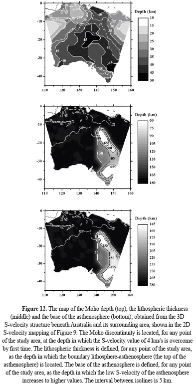
Depth range: 15 - 50 km. The geographical distribution of the S-velocity values for this depth range shows higher values (4 km/s and higher) in zones of the study area in which the Moho depth is overcome (i. e. zones which the depth range considered is located below the Moho discontinuity). For each depth range shown in Figura 9 (between 15 and 50 km), the Moho depth is overcome in different areas. The Moho depth is firstly overcome in off-shore areas and lastly in on-shore and continental areas. In general, the S-velocity increases with depth for the whole study area, as shown by Figura 9, for each depth range between 15 and 50 km. Again, the S-velocity presents the lowest values at the east of the Tasman Line, while the highest ones are present at the west of this line. This feature doesn't appear in the S-velocity mapping performed by Saygin and Kennett (2012). For this depth range, there is no S-velocity change associated with the Tasman Line, in their mapping. The S-velocity presents higher values for the consolidated and old structures. Nevertheless, the S-velocity difference associated with this structural difference is minor than the S-velocity difference due to the Moho depth overcoming, because the S-velocities associated with the crust are much minor than those associated with the upper mantle. The results obtained for this depth range (from 15 to 50 km) agree well with those obtained by Ellis and Denham (1985) and Denham and Ellis (1986). Although, the few seismic paths considered by them only allow the determination of media values for the Moho depth, which agree well with the Moho map obtained in the present study (Figure 12). In the present study, an S-velocity value greater than 4 km/s is considered associated with the upper-mantle structure. Thus, if the S-velocity value of 4 km/s is used to find the Moho depth in the whole study area, considering that an S-velocity value greater than 4 km/s is associated with upper-mantle structure, then it is possible to plot a map of the Moho discontinuity, such as the map shown in Figure 12 (top), from the S-velocity mapping shown in Figura 9 (which is in fact an ensemble of 2D plots for a 3D S-velocity distribution). This Moho map agrees well with other Moho maps previously calculated for Australia, as the Moho maps obtained by Aitken (2010), Kennett et al. (2011), Kennett and Salmon (2012) and Saygin and Kennett (2012). It is very noticeable that the most recent maps calculated for Australia (Kennett and Salmon, 2012; Saygin and Kennett, 2012) are very similar to AusMoho (Kennett et al., 2011), as consequence of the use of similar databases for their calculation. Thus, a comparison of the Moho map shown in Figure 12 (top) with anyone of them gives the same.

Depth range: 50 - 65 km. Again, the S-velocity presents the highest values at the west of the Tasman Line (Figure 11), while the S-velocity values at the east of the Tasman Line are the lowest ones. Moreover, the S-velocity presents higher values for the consolidated and old structures, which allows the identification, in terms of S-velocity, of the principal units that compose Australia. On the other hand, the S-velocity values calculated for the northern part of the study area (the south of Indonesia and the surrounding seas) agree well with those obtained by Okabe et al. (2004). Nevertheless, a better resolution is achieved in the present study, because they divide the study area in blocks with 5°×5° in size, while this area is gridded with 2.5°×2.5° mesh size in the present study. A comparison with previous studies developed in the Australian continent is not possible, because no 3D S-velocity structure was obtained for depths ranging from 30 to 75 km. The results obtained in this study, for this depth range, are a new and very interesting feature never presented before.

Depth range: 65 - 80 km. The S-velocity pattern shown is similar to that in the previous depth range, except for the south-eastern and north-eastern parts of Australia, in which the S-velocity shows lower values. Fishwick and Reading (2008) confirmed this pattern of low velocities for south-eastern and north-eastern parts of Australia. Also, Fishwick and Rawlinson (2012) confirmed with their results that the S-velocity values, at the east of the Tasman Line, are the lowest obtained for Australia. Moreover, the results obtained by them, for the whole study area (Australia and its surrounding area), agree well with those obtained in the present study, although the resolution achieved in the present study is the best. On the other hand, the S-velocity shows low values in the south-eastern and north-eastern parts of Australia, because the asthenosphere is reached at this depth range (from 65 to 80 km) and for these areas, as shown in Figure 12 (middle). The lithosphere-asthenosphere boundary (or equivalently the lithosphere thickness) shown in Figure 12 (middle), has been computed from the 3D S-velocity structure, calculated in the present study and represented by the 2D S-velocity mapping shown in Figura 9, considering for each point of the study area the depth in which the S-velocity starts to decrease with depth. The lithosphere thickness map shown in Figure 12 (middle) agrees well with the lithosphere-asthenosphere boundary (LAB), obtained by Ford et al. (2010) from Sp wave imaging. Nevertheless, a better resolution is achieved in the present study because they interpret a strong coherent negative Sp phase in eastern Australia as the LAB, but no tomography is performed in their study. Also, a better resolution is achieved for the LAB in Figure 12 (middle) comparing with that performed by Kennett and Salmon (2012).

Depth range: 80 - 105 km. The S-velocity pattern shown is similar to that in the previous depth range, except for the north-eastern part of Australia, in which the zone of lower S-velocity is increased respect to the previous depth range, because the asthenosphere is reached, at this depth range, for a wider zone of the north-east of Australia, as shown in Figure 12 (middle). This feature is confirmed by the LAB obtained by Ford et al. (2010) and is also confirmed by previous studies (Zielhuis and van der Hilst, 1996; Simons et al., 1999; Fishwick et al., 2005; Fishwick and Reading, 2008; Fichtner et al., 2009; Fishwick and Rawlinson, 2012). The results obtained in these previous studies also agree well with those obtained in the present study, for the whole study area. Concretely, all S-velocity maps calculated in the studies performed until now (including the present study), show high values of S-velocity at the west of the Tasman Line (Figure 11), while the S-velocity values at the east of the Tasman Line are the lowest ones. Moreover, the S-velocity presents higher values for the consolidated and old structures. Nevertheless, the identification of the principal units that compose Australia, in terms of S-velocity, is clearer in the S-velocity maps of the present study than in those of any previous study. On the other hand, the S-velocity values calculated for the northern part of the study area (the south of Indonesia and the surrounding seas), in the present study, are higher in the northwest than in the northeast. Although, in the S-velocity map of present depth range (from 80 to 105 km), appears a zone of high velocity in the north-eastern part of the study area. This high S-velocity also appears in the same zone of the S-velocity maps obtained by Fichtner et al. (2009), for the depths of 80 and 110 km. These S-velocity values agree well with those obtained by Okabe et al. (2004). Nevertheless, a low resolution of their maps (they divide the study area in blocks with 5°×5° in size) makes difficult the comparison with the results of the present study.

Depth range: 105 - 130 km. The S-velocity pattern shown is similar to that in the previous depth range, except for the eastern part of Australia, in which the S-velocity shows the lowest values, because the asthenosphere is reached, at this depth range and for this area, as shown in Figure 12 (middle). Again, this feature is confirmed by the LAB obtained by Ford et al. (2010) and is also confirmed by other studies (Zielhuis and van der Hilst, 1996; Simons et al., 1999; Fishwick et al., 2005; Fishwick and Reading, 2008; Fichtner et al., 2009; Fishwick and Rawlinson, 2012; Kennett and Salmon, 2012). Nevertheless, the identification of the principal units that compose Australia, in terms of S-velocity, is again clearer in the S-velocity maps of the present study than in those of any previous study. Also, for the present depth range, the S-velocity values calculated for the northern part of the study area agree well with those obtained by Okabe et al. (2004), although, the low resolution of their maps makes difficult the performing of a precise comparison.

Depth range: 130 - 155 km. The S-velocity pattern shown is similar to that in the previous depth range, except for the central-eastern part of Australia (from the Tasman Line toward east, approximately), in which the S-velocity shows the lowest values, because the asthenosphere is reached, at this depth range and for this area, as shown in Figure 12 (middle). Again, this feature is confirmed by the LAB obtained by Ford et al. (2010), which is also in agreement with the S-velocity distributions with depth shown in Figure 13, for perpendicular cross-sections along the parallels of 25 and 30°S. These cross-sections have been obtained from the 3D S-velocity structure calculated in the present study, by vertical interpolation from the 2D S-velocity mapping shown in Figura 9. It should be noted that the cross-sections obtained in the present study show a better resolution than those obtained by Fichtner et al. (2009), for depths greater than 250 km. This improvement in the resolution at the deeper depths achieved in this study is related to the wide period range, in which the Rayleigh-wave group velocities have been measured. In the present study, dispersion curves (group velocities) until 250 s of period have been determined, providing observed data to fit the deep S-velocity structure with more accuracy than any previous studies.

Depth range: 155 - 180 km. The S-velocity pattern shown is similar to that in the previous depth range, except for the north-eastern and south-eastern parts of Australia, in which the S-velocity shows higher values comparing with those in the previous depth range, because the asthenosphere is overcome, at this depth range and for these areas, as shown in Figure 12 (bottom). The boundary of the asthenosphere base (or equivalently the lithosphere-asthenosphere system thickness) shown in Figure 12 (bottom), has been computed from the 3D S-velocity structure, calculated in the present study and represented by the 2D S-velocity mapping shown in Figura 9, considering for each point of the study area the depth in which the S-velocity starts to increase with depth below the LAB. It was found that the map of asthenosphere base, shown in Figure 12 (bottom), is a new and very interesting feature never obtained before the present study. Also, it is very noticeable that the mantle low-velocity zone (i. e. the asthenosphere), identified in Australia from the LAB (Figure 12 middle) to the asthenosphere base (Figure 12 bottom), is shallower for the eastern part of Australia, at the east of the Tasman Line, coinciding with the Australian region of higher heat flow (Cull, 1982). This increment in the heat flow, found at the east of the Tasman Line, could be originated precisely by an asthenosphere nearer to earth surface, for the eastern part of Australia (i. e. a thinness of the lithosphere towards the east from the Tasman Line). Fishwick et al. (2008) have presented evidence for the progressive eastward thinning of the lithosphere across Australia. This behaviour is also confirmed by Kennet and Salmon (2012), who have observed that the dominant control on the seismic velocities in the mantle is from temperature, with a decreasing in velocity associated with the increasing in temperature. They suggest that the variations in the seismic velocity with depth can be interpreted in terms of changes in the lithospheric thickness (i. e. variations on the asthenosphere depth). Thus, the regions, in which are present consolidated and old structures characterized by higher S-velocities (located at the west of the Tasman Line), are underlain by a thick mantle lithosphere, while the lithosphere is generally thinner beneath the regions at the east of the Tasman Line, characterized by lower S-velocities. This shallower part of the asthenosphere is particularly the shallowest part for the eastern margin of Australia (i. e. the thinnest lithosphere), coinciding with the sites of Cenozoic volcanism (Johnson, 1989). On the other hand, a low-velocity zone is also present, for a similar depth range, in the mantle of the continents: South America (Corchete, 2012), Antarctica (Corchete, 2013a) and Africa (Corchete, 2013b), which were part of the same super-continent Gondwanaland (Supplement 7), in the early Mesozoic before fragmentation. This new and very interesting feature proves that it is possible the precise reconstruction of Gondwanaland, comparing the high and low velocity areas found in South America, Antarctica, Africa and Australia.

Depth range: 180 - 230 km. The S-velocity pattern shown is very different from that in the previous depth range, because the asthenosphere is reached for the major part of the study area, as shown in Figure 12 (middle), except for the north-eastern and south-eastern parts of Australia, in which the asthenosphere was overcome for the previous depth range. Opposite to this, the asthenosphere is overcome for the eastern part of Australia, as shown in Figure 12 (bottom). For this reason, the S-velocity shows higher values (for this area and for the present depth range) comparing with those shown for the previous depth range, but in general, the S-velocity (in the present depth range) presents values lower than those shown the previous depth range, for the major part of the study area, as a consequence of the asthenosphere presence in the major part of the study area. This feature is also shown in Figure 13 and confirmed by the LAB obtained by Ford et al. (2010). On the other hand, they have obtained that the LAB is defined by a sharp discontinuity in the eastern part of Australia, while this boundary is gradual in the western part of this continent. This feature is confirmed by Kennet and Salmon (2012), who have found that the lithosphere beneath the older parts of the continent can be readily recognised by fast S-velocities, but the transition to the asthenosphere is not marked by any sharp transition. This behaviour is also shown in Figure 13, because the S-velocity decreases gradually with depth (from 180 to 280 km) in the western part of Australia, while the S-velocity distribution with depth shows a sharp LAB in the eastern part of Australia. This LAB is located at different depths for eastern part of Australia, as shown in Figure 12 (middle).

Depth range: 230 - 280 km. The S-velocity pattern shown is similar to that in the previous depth range, because the asthenosphere was reached for the major part of the study area in the previous depth range. Opposite to this, the asthenosphere is overcome for the central-eastern part of Australia (from the Tasman Line toward east, approximately), as shown in Figure 12 (bottom). For this reason, the S-velocity shows higher values (for this area and for the present depth range) comparing with those shown for the previous depth range. Nevertheless, the S-velocity in the depth range from 230 to 280 presents the lowest values calculated for the study area, comparing with those calculated for the depth range from 50 to 400 km (Figura 9). This feature can be more clearly observed in Figure 13, in which the depth range from 230 to 280 presents, in general, the lowest values of S-velocity. Previous studies (Simons et al., 1999; Fishwick et al., 2005; Fishwick and Reading, 2008; Fichtner et al., 2009; Fishwick and Rawlinson, 2012; Kennet and Salmon, 2012) also obtained the lowest S-velocity values for this depth range, but the resolution of these previous studies is poorer than that from the present study, for depths greater than 250 km. The improvement in the resolution at the deeper depths achieved in this study is related to the wide period range, in which the Rayleigh-wave group velocities have been measured. In the present study, dispersion curves (group velocities) until 250 s of period have been determined, providing observed data to fit the deep S-velocity structure with more accuracy than the above-mentioned previous studies.

Depth range: 280 - 400 km. The S-velocity values shown in Figura 9 jump respect to those shown in the previous depth range, from low values (4.2 - 4.4 km/s) to high values (4.8 - 5.1 km/s). This jump of the S-velocity, at this depth range, can be more easily observed in both cross-sections of Figure 13. Obviously, the low-velocity channel associated with the asthenosphere, shown in the previous depth range, has been overcome for the whole study area in the present depth range. Again, the S-velocity presents the highest values at the west of the Tasman Line (Figure 11), while the S-velocity values at the east of the Tasman Line are the lowest. Moreover, the S-velocity presents higher values for the consolidated and old structures, but the identification, in terms of S-velocity, of the principal units that compose Australia is more difficult for this deeper depth range, because the S-velocity differences are very little for this depth range. The S-velocity contrast decreases with depth while the S-velocity values increase with depth, obtaining an S-velocity pattern of similar high S-velocity values, for the whole study area. Thus, at the opposite of the results obtained in the previous depth ranges, the S-velocity remains almost the same with depth, for the whole study area. This pattern of high velocities also have been obtained beneath Australia, for this depth range, in other previous studies (Simons et al., 1999; Fishwick et al., 2005; Fishwick and Reading, 2008; Fichtner et al., 2009; Fishwick and Rawlinson, 2012; Kennet and Salmon, 2012) but their resolution is very low at these deeper depths, which makes it difficult to compare the results of these previous studies, with those obtained in the present study. On the other hand, a similar smooth correlation between older (or more consolidated) structures and high S-velocity values has been found (at this depth range) for the continents: South America (Corchete, 2012), Antarctica (Corchete, 2013a) and Africa (Corchete, 2013b), which were part of the same super-continent Gondwanaland. This new and very interesting feature proves again that it is possible the precise reconstruction of old super-continents (now fragmented), comparing the high and low velocity areas present in the modern continents.

7. Conclusions

The results presented in this paper show that the techniques used here are a powerful tool for investigating the elastic structure of Earth. This methodology that is a good tool to investigate the physical properties of the earth structure, in any region of Earth with a variety of tectonic features, has been improved in the present paper performing a new method for the regionalization of surface-wave dispersion, based on Fourier series, never published before in any previous paper. By means of this analysis, the principal structural features beneath Australia and its surrounding area have been revealed. Such features include the existence of lateral and vertical heterogeneity in the whole study area, which is concluded in Figures 9, 12 and 13. The zones with consolidated and old structures present higher S-velocity values than the other zones (which allows the identification of the principal geological units of Australia, in terms of S-velocity), although this difference can be negligible in some cases (e. g. for depths greater than 280 km). Nevertheless, in the depth range of 15 to 50 km, the different Moho depths present in the study area generate the principal variation of S-velocity, because the S-velocities associated with the crust are less than those associated with the upper mantle. A similar behaviour is found for the LAB, which generates the principal variations of S-velocities in the depth range from 65 to 180 km, because the S-velocities associated with the lithosphere are much major than those associated with the asthenosphere, as is well known. On the other hand, a new and interesting feature, obtained in this study, is the definition of the base of the asthenosphere, for the whole study area, for depths ranging from 155 to 280 km. This boundary joint to the LAB define a low-velocity zone in the Australian mantle, which is also present for a similar depth range in the continents (South America, Antarctica and Africa) that were part of the same super-continent Gondwanaland.

Acknowledgements. The author is grateful to the Incorporated Research Institutions for Seismology (IRIS), for providing data used in this study. The seismograms and the instrumental response have been provided by IRIS, through the internet utility WILBER II and the database: IRIS DMC MetaData Aggregator (available at www.iris.edu), respectively. The author is also grateful to the international and local agencies (and persons), who have been able to develop and support the seismic stations (portable deployments within Australia and permanent installations), which data has been used in this study.

---

References

Aitken A., 2011. Moho geometry gravity inversion experiment (MoGGIE): A refined model of the Australian Moho, and its tectonic and isostatic implications. Earth and Planetary Science Letters, 297, 71-83.

Aki K. and Richards P. G., 1980. Quantitative Seismology. Theory and methods. W. H. Freeman and Company, San Francisco.

Cara M., 1973. Filtering dispersed wavetrains. Geophysical Journal of the Royal Astronomic Society, 33, 65-80.

Corchete V., Chourak M. and Hussein H. M., 2007. Shear wave velocity structure of the Sinai Peninsula from Rayleigh wave analysis. Surveys in Geophysics, 28, 299-324.

Corchete V. and Chourak M., 2010. Shear-wave velocity structure of the western part of the Mediterranean Sea from Rayleigh-wave analysis. International Journal of Earth Sciences, 99, 955-972.

Corchete V., 2012. Shear-wave velocity structure of South America from Rayleigh-wave analysis. Terra Nova, 24, 87-104.

Corchete V., 2013a. Shear-wave velocity structure of Antarctica from Rayleigh-wave analysis. Tectonophysics, 583, 1-15.

Corchete V., 2013b. Shear-wave velocity structure of Africa from Rayleigh-wave analysis. International Journal of Earth Sciences, 102, 857-873.

Cull J. P., 1982. An appraisal of Australian heat flow data. Bureau of Mineral Resources Journal of Australian Geology and Geophysics, 7, 11-21.

Denham D. and Ellis R. M., 1986. Determination of earthquake focal mechanisms and crustal structure in eastern Australia using surface waves. Tectonophysics. 121, 109-123.

Dziewonski A., Bloch S., and Landisman M., 1969. A technique for the analysis of transient seismic signals. Bulletin of the Seismological Society of America, 59, No. 1, 427-444.

Dziewonski A. M. and Anderson D. L., 1981. Preliminary reference earth model. Physics of the Earth and Planetary Interiors, 25, 297-356.

Ellis R. M. and Denham D., 1985. Structure of the crust and upper mantle beneath Australia from Rayleigh- and Love-wave observations. Physics of the Earth and Planetary Interiors, 38, 224-234.

Fichtner A., Kennett B. L. N., Igel H. and Bunge H-P, 2009. Full seismic waveform tomography for upper-mantle structure in the Australasian region using adjoint methods. Geophysical Journal International, 179, 1703-1725.

Fishwick S., Kennett B. L. N. and Reading A. M., 2005. Contrasts in lithospheric structure within the Australian craton-insights from surface wave tomography. Earth and Planetary Science Letters, 231, 163-176.

Fishwick S., Heintz M., Kennett B. L. N., Reading A. M. and Yoshizawa K., 2008. Steps in lithospheric thickness within eastern Australia, evidence from surface wave tomography. Tectonics, 27, doi: 10.1029/2007TC002116.

Fishwick S. and Reading A. M., 2008. Anomalous lithosphere beneath the Proterozoic of western and central Australia: A record of continental collision and intraplate deformation? Precambrian Research, 166, 111-121.

Fishwick S. and Rawlinson N., 2012. 3-D structure of the Australian lithosphere from evolving seismic datasets. Australian Journal of Earth Sciences, 59, 809-826.

Ford H. A., Fischer K. M., Abt D. L., Rychert C. A. and Elkins-Tanton L. T., 2010. The lithosphere-asthenosphere boundary and cratonic lithospheric layering beneath Australia from Sp wave imaging. Earth and Planetary Science Letters, 300, 299-310.

Johnson R.W. (ed.), 1989. Intraplate volcanism in Eastern Australia and New Zealand. Cambridge University Press, Melbourne.

Keilis-Borok V. I., 1989. Seismic surface waves in a laterally inhomogeneus Earth. Kluwer Academic Publishers, London, UK.

Kennett B. L. N., Salmon M., Saygin E. and AusMoho Working Group, 2011. AusMoho: the variation of Moho depth in Australia. Geophysical Journal International, doi: 10.1111/j.1365-246X.2011.05194.x.

Kennett B. L. N. and Salmon M., 2012. AuSREM: Australian Seismological Reference Model. Australian Journal of Earth Sciences, accepted.

Okabe A., Kaneshima S., Kanjo K., Ohtaki T. and Purwana I., 2004. Surface wave tomography for southeastern Asia using IRIS-FARM and JISNET data. Physics of the Earth and Planetary Interiors, 146, 101-112.

Roult G. and Rouland D., 1994. Antarctica I: Deep structure investigations inferred from seismology; a review. Physics of the Earth and Planetary Interiors, 84, 15-32.

Saygin E. and Kennett B. L. N., 2012. Crustal structure of Australia from ambient seismic noise tomography. Journal of Geophysical Research, 117, B01304, doi: 10.1029/2011JB008403.

Simons F. J., Zielhuis A. and van der Hilst R. D., 1999. The deep structure of the Australian continent from surface wave tomography. Lithos, 48, 17-43.

Zielhuis A. and van der Hilst, R. D., 1996. Upper-mantle shear velocity beneath eastern Australia from inversion of waveforms from SKIPPY portable arrays. Geophysical Journal International, 127, 1-16.