Uncertainty in rainfall input data in a conceptual water balance model: effects on outputs and implications for predictability

As hydrological models become more prevalent in water resources planning and management, increasing levels of detail and precision are needed. Currently, reliable models that simulate the hydrological behavior of a basin are indispensable; however, it is also necessary to know the limits of the predictability and reliability of the model outputs. The present study evaluates the influence of uncertainty in the main input variable of the model, rainfall, on the output uncertainty of a hydrological model. Using concepts of identifiability and sensitivity, the uncertainty in the model structure and parameters was estimated. Then, the output uncertainty caused by uncertainties in i) the rainfall amounts and ii) the periods of the rainfall was determined. The main conclusion is that uncertainty in rainfall estimation during rainy periods produces greater output uncertainty. However, in non-rainy periods, the output uncertainty is not very sensitive to the uncertainty in rainfall. Finally, uncertainties in rainfall during the basin filling and emptying periods (Apr. – Jun. and Sep. – Nov., respectively) alter the uncertainty in subsequent periods. Therefore, uncertainties in these periods could result in limited ranges of model predictability.

Los modelos hidrológicos se han vuelto cada vez más necesarios en la planificación y gestión de recursos hídricos, donde un aumento en los niveles de detalle y precisión es necesario. Actualmente disponer de modelos para simular el comportamiento hidrológico de una cuenca resulta indispensable, sin embargo, también es necesario conocer los límites de predictibilidad y de confiabilidad de las salidas de un modelo. En este estudio se evalúan la influencia de la incertidumbre en la principal entrada de un modelo, la precipitación, sobre la incertidumbre de las salidas de un modelo hidrológico. Utilizando conceptos de identificabilidad y sensibilidad se estima la incertidumbre de los parámetros y estructura de un modelo. Luego, la incertidumbre en las salidas causadas por incertidumbre en i) los montos de precipitación, ii) los períodos de precipitación fue calculada. Como conclusiones se obtuvo que la incertidumbre en la estimación de la precipitación en períodos de lluvia produce mayor incertidumbre sobre las salidas. En períodos no lluviosos, la incertidumbre de las salidas es poco sensible a incertidumbre sobre las precipitaciones. Finalmente, incertidumbres en periodos de llenado y vaciado (Abril-Junio y Septiembre-Noviembre respectivamente) afectan la incertidumbre en las salidas en los períodos subsecuentes. Por lo tanto incertidumbres en aquellos períodos pueden resultar en rangos limitados de predictibilidad de un modelo.

METEOROLOGY

Enrique Muñoz, Pedro Tume, Gabriel Ortíz¹

1. Alonso de Ribera 2850, Concepción. Departamento de Ingeniería Civil, Universidad Católica de la Santísima Concepción, Concepción, Chile

E-mail: emunozo@ucsc.cl, ptume@ucsc.cl, gaortiz@ing.ucsc.cl

Record
Manuscript received: 16/07/2013 Accepted for publication: 29/04/2014

---

ABSTRACT

As hydrological models become more prevalent in water resources planning and management, increasing levels of detail and precision are needed. Currently, reliable models that simulate the hydrological behavior of a basin are indispensable; however, it is also necessary to know the limits of the predictability and reliability of the model outputs. The present study evaluates the influence of uncertainty in the main input variable of the model, rainfall, on the output uncertainty of a hydrological model. Using concepts of identifiability and sensitivity, the uncertainty in the model structure and parameters was estimated. Then, the output uncertainty caused by uncertainties in i) the rainfall amounts and ii) the periods of the rainfall was determined. The main conclusion is that uncertainty in rainfall estimation during rainy periods produces greater output uncertainty. However, in non-rainy periods, the output uncertainty is not very sensitive to the uncertainty in rainfall. Finally, uncertainties in rainfall during the basin filling and emptying periods (Apr. – Jun. and Sep. – Nov., respectively) alter the uncertainty in subsequent periods. Therefore, uncertainties in these periods could result in limited ranges of model predictability.

Key words: Uncertainty, hydrological predictability, surface hydrology, water resources.

RESUMEN

Los modelos hidrológicos se han vuelto cada vez más necesarios en la planificación y gestión de recursos hídricos, donde un aumento en los niveles de detalle y precisión es necesario. Actualmente disponer de modelos para simular el comportamiento hidrológico de una cuenca resulta indispensable, sin embargo, también es necesario conocer los límites de predictibilidad y de confiabilidad de las salidas de un modelo. En este estudio se evalúan la influencia de la incertidumbre en la principal entrada de un modelo, la precipitación, sobre la incertidumbre de las salidas de un modelo hidrológico. Utilizando conceptos de identificabilidad y sensibilidad se estima la incertidumbre de los parámetros y estructura de un modelo. Luego, la incertidumbre en las salidas causadas por incertidumbre en i) los montos de precipitación, ii) los períodos de precipitación fue calculada. Como conclusiones se obtuvo que la incertidumbre en la estimación de la precipitación en períodos de lluvia produce mayor incertidumbre sobre las salidas. En períodos no lluviosos, la incertidumbre de las salidas es poco sensible a incertidumbre sobre las precipitaciones. Finalmente, incertidumbres en periodos de llenado y vaciado (Abril-Junio y Septiembre-Noviembre respectivamente) afectan la incertidumbre en las salidas en los períodos subsecuentes. Por lo tanto incertidumbres en aquellos períodos pueden resultar en rangos limitados de predictibilidad de un modelo.

Palabras clave: Incertidumbre, predictibilidad hidrológica, hidrología superficial, recursos hídricos.

---

INTRODUCTION

Considering that i) water is a limited resource, ii) its demand increases with development and population growth, iii) its availability changes year to year due to local, global, natural and anthropogenic phenomena, iv) the impact of climate change on the water supply is of fundamental importance and v) a large part of the world's population is already experiencing water stress (Vörösmarty et al., 2000), it is necessary to develop tools for efficient water resources management and to support the prediction of future conditions under different scenarios caused by local (orographic), regional (El Niño Southern Oscillation) or global effects (climate change).

One alternative for efficient water resources management and planning is the use of hydrological models. A model attempts to reproduce a physical phenomenon that occurs in an object or area. Therefore, in hydrology, a model seeks to represent an area defined by a watershed, the phenomena of rainfall-runoff processes and the associated water movement. The objective of reproducing these processes is to simulate and predict future conditions for management, administration and optimization of water uses. Consequently, it is essential to have reliable models that adequately represent the hydrological behavior of a basin. For example, when using predictive models or alternative sources of information (e.g., global datasets) (Mahe et al., 2008, Muñoz, 2010), it is necessary to know the predictability limits of the model outputs and their uncertainty.

Normally, a conceptual hydrological model requires at least two input variables (potential evapotranspiration and rainfall) to quantify the inputs and water losses in the water balance. Rainfall is the main input variable for a hydrological model (Olsson and Lindström, 2008). Therefore, the potential predictability and the range of the predictability of the basin flows depend on the uncertainty associated with the input variables and their quality.

Uncertainty is defined as the degree of the lack of knowledge of or confidence in a certain process or result (Caddy and Mahorn, 1995). Therefore, in a hydrological model, the sources of uncertainty are associated with the input variables (lack of knowledge of the quality of the measurements and predictions) and with the model structure and calibration parameters (lack of knowledge and simplification of the simulated hydrological processes in a basin). The present study aims to quantify how uncertainty in the outputs of a conceptual hydrological model is affected by uncertainty in the main input, rainfall, while keeping the uncertainty associated with the model structure and calibration parameters fixed.

METHODS

Case Study

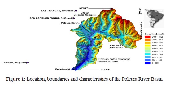
The Polcura River Basin (Figure 1) is located in the temperate zone of South-Central Chile, between 37°20'S - 71#º31'W and 36°54'S - 71°06'W. It is bounded by the Andes to the east, the Nevados de Chillán volcanic complex to the north, and Lake Laja to the south. It comprises an area of 914 km² that is between 700 and 3,090 masl; the area is characterized by steep slopes (≈ 26° on average) that are mainly composed of partially eroded volcano-sedimentary sequences (OM2c, PPl3 and M3i) (SERNAGEOMIN, 2006).

In addition, the area is located in an extratropical zone that is greatly affected by El Niño Southern Oscillation (ENSO) (Grimm et al., 2000), which introduces seasonality and interannual variability to the local hydro-meteorological patterns (Grimm et al., 2000; Montecinos and Aceituno, 2003).

The average annual precipitation in the basin is 2300 mm, with a pluvial period during winter and an ice-melt and snowmelt period in spring and early summer. The average monthly temperature is 9° C, ranging from 2.5° C in winter to 16.5 ° C in summer.

Because of the location of the basin, its mountainous nature and its geomorphology (Figure 1), it exhibits high temporal variability with respect to hydro-meteorological characteristics, where the orographic effect on the eastern slope of the Andes produces an increase in rainfall (Garreaud, 2009; Vicuña et al., 2011). Additionally, the area is affected by ENSO. ENSO is a coupled ocean-atmosphere phenomenon that is characterized by irregular periodicity (2 to 7 years), where the alternation between El Niño and La Niña episodes is associated with above and below average rainfall and warmer and colder than normal air temperatures, respectively (Garreaud, 2009).

Therefore, the characteristics of the basin, such as high rainfall variability and ENSO effects, provide an ideal case study in which uncertainty in precipitation could be the main source of uncertainty in predictions.

Description of the water balance model

The model used in this paper is the snow-rain conceptual water balance model presented by Muñoz (2010) and Muñoz et al. (2014). This model separately simulates pluvial and snow-melting processes and includes external alterations, such as irrigation or transfer canals, by adding or subtracting flows. This model has been successfully implemented in Andean basins in South-Central Chile (e.g., Zúñiga et al., 2012, Arumí et al., 2012). Therefore, it is an adequate option for analyzing the study area.

The pluvial component is modeled using a lumped monthly rainfall-runoff model that treats the watershed as a double storage system: subsurface (SS) and underground storage (US). SS represents the water stored in the unsaturated soil layer as soil moisture. US is the water that covers the saturated soil layer. The model requires two inputs: rainfall (PM) and potential evapotranspiration (PET). The model output is the total runoff (ETOT) at the watershed outlet, and it includes both subterranean (ES) and direct runoff (EI). These amounts are calculated by six calibration parameters and two input modifiers (useful in case of non-representative PM and PET data).

The snowmelt model calculates snowfall (Psnow) based on precipitation above the 0 (°C) isotherm. Psnow is stored in the snow storage system (SN), for which the melting calculations are performed using the degree-day method (Rango and Martinec, 1995). Thus, potential melting (PSP) is estimated, and depending on the snow stored, real melting (PS) is calculated. Then, PS is distributed in the pluvial model through calibration parameter F.

Every calibration parameter has a conceptual meaning for integrating spatial and temporal variability. Table 1 presents a brief description of the model parameters and their influence on the model.

The external alterations module permits the incorporation of alterations, such as irrigation or transfer canals, and simulates inflows and/or outflows to/from the basin by adding or subtracting flows as follows:

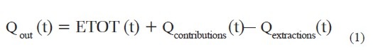
where the basin outflow (Qout) at time t is the basin runoff (ETOT) plus the contributions (Qcontributions) and less the extractions (Qextractions) during the same period. For a further explanation of the model, refer to Muñoz (2010) and Muñoz et al. (2014).

Model inputs

To run the described model, it is necessary to obtain precipitation, temperature and potential evapotranspiration series, as well as the geomorphological characterization of the basin to compute the monthly 0°C isotherm elevation.

For the geomorphological characterization of the basin, a digital elevation model was constructed using data from the Shuttle Radar Topography Mission (SRTM) of 3 arc-seconds (90 m). For the inputs, rainfall series from the rain gauge stations of Las Trancas, San Lorenzo and Trupán were obtained (administered by the Dirección General de Aguas, DGA). Temperature series from the Center for Climatic Research of the University of Delaware (UD) (Willmot and Matsuura, 2008) were collected. Climatological model inputs were constructed using both sources of information. Additionally, the potential evapotranspiration series were calculated using the Thornthwaite method and the UD temperature data series. The spatial distribution of these variables in the basin was determined using Thiessen polygons. Based on prior experience, both the Thornthwaite and Thiessen polygons methods are adequate for estimating potential evapotranspiration and for determining the meteorological spatial distribution of monthly data in basins of South-Central Chile (e.g., Muñoz, 2010, Zúñiga et al., 2012). Therefore, both methods were used in this study.

Because of the availability and quality of the input data, the analysis was performed on a monthly scale for a period of 13 years (1990 – 2002). The stream gauge station for controlling the basin outflows is the Polcura Antes de Descarga central El Toro station (Figure 1).

Uncertainty analysis

To quantify the uncertainty, the Monte Carlo Analysis Toolbox (MCAT) (Wagener and Kollat, 2007) was used. MCAT is a tool that operates under the Generalized Likelihood Uncertainty Estimation methodology (Beven and Binley, 1992), and it contains a group of analysis tools to explore the identifiability of a model and its parameters. MCAT was chosen because it is an easy-to-use tool and is an adequate and simple option for evaluating model behavior and uncertainty.

To evaluate identifiability and quantify the uncertainty in a model, MCAT operates by performing repetitive simulations using a set of randomly selected parameters within a range defined by the user. The program stores the outputs and values of the objective function(s) for subsequent analyses. In this case, due to the lack of knowledge of the parameter distribution, a prior uniform distribution of the model parameters was used.

Parameters of hydrological models cannot be identified as unique sets of values. This is mainly because changes in one parameter can be compensated by changes in one or more other parameters due to their interdependence (Bárdossy, 2007) and because the processes simulated in a hydrological model are commonly interrelated. In the case of the Muñoz (2010) model, for example, direct runoff depends on Cmax; therefore, the processes that occur in the subsurface storage layer depend on the amount of rainfall that is not transformed into runoff (i.e., 1-Cmax); consequently, the processes that occur in this storage layer depend on the identifiability of Cmax. This generates an interconnection among the identifiability of the calibration parameters of a model. Therefore, it is necessary to perform various iterations as a means of restricting the range of the validity of the parameters that first show identifiability and to observe identifiability in the remaining (dependent) parameters as a means of reducing the identifiability range of these parameters.

Because the Monte Carlo method is based on random trials, it normally requires a large number of simulations that cover a wide spectrum of possible simulations. In this case, the number of Monte Carlo simulations was estimated via trial and error. The "stop" criterion was met when the correlation (according to the Pearson correlation coefficient) between uncertainty bands (calculated as a linear correlation between the time series of the upper and lower limits of the uncertainty bands) of two trials with the same number of simulations was equal to or greater than 0.999. Under this criterion, it was determined that the adequate number of simulations for this study was 25,000.

The procedure to estimate the rainfall uncertainty and to differentiate it from the model structure and calibration parameters was as follows:

Through an identifiability analysis of the factors for the modification of the inputs (a comparison of these factors with the value of the objective function), these factors were limited to precise values. It is necessary to set these factors to unique values, as they ensure the long-term water balance in which the precipitation input volumes are equal to the evapotranspiration and flow output volumes during the entire period of the simulation.

With the values of these fixed factors, new simulations were performed, in which the ranges of variation assigned to each parameter were reduced in accordance with the observed identifiability. The established stop criterion was defined as when identifiability was not observed in the new defined range (the reduced range) of each parameter.

After the identifiability analysis, the resulting uncertainty in the model outputs was quantified. This uncertainty was defined as the uncertainty associated with the model structure and calibration parameters.

The confidence level was 90% (a range between 5 and 95% of the outputs for each time step of the series). The established rejection criterion was set according to the Kling-Gupta efficiency objective function (KGE) (Gupta et al., 2009). The KGE function (Eq. 2) is an improvement of the Nash-Suctliffe efficiency index (NSE) (Nash and Sutcliffe, 1970) in which correlation, deviation and variability are equally weighted to resolve systematic underestimation of the maximum values and low variability identified in the NSE function (Gupta et al., 2009). The KGE varies between - ∞ and 1, where the best model is closest to 1. Because the GLUE methodology is based on likelihood, the KGE was transformed into 1-KGE. With this change, 1-KGE represents a measure of likelihood in which the best model is closest to 0 and the worst model is + ∞.

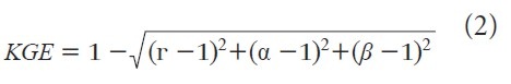
where r is the linear correlation between the simulated and observed flows, α is the ratio between the standard deviation of the simulated and observed flows and represents the variability in the values, and β is the ratio between mean simulated and mean observed flows (i.e., the bias).

Then, with the uncertainty associated with the model structure and parameters quantified, the rainfall series were modified for different magnitudes and periods, as shown in Table 2. It is important to note that this variation corresponds to a punctual variation of the rainfall series of different magnitudes and periods, and uncertainty is not added as a rainfall range in each time step. This analysis aims to identify how output uncertainty would be affected by an error in the precipitation prediction.

RESULTS AND DISCUSSION

Using the previously described methods, uncertainty associated with the model structure and parameters was found; then, the uncertainty related to rainfall data were computed and analyzed. The major findings and a discussion are presented as follows.

Uncertainty associated with model structure and calibration parameters

Figure 2 shows the identifiability and sensitivity analysis performed for the model parameters. The graphs show the probability distribution function (pdf) and the cumulative distribution function (cdf) of each parameter for the best 10% of the simulations according to a determined objective function (KGE in this case).

As observed, five parameters presented identifiability (according to the pdf): A, B, Cmax, Hmax and Ck. According to the cdf, A, Cmax and Ck were the most sensitive (i.e., greater slope within a determined range) to the model outputs.

Because of the identifiability analysis, the ranges of variations in these five identifiable model parameters were reduced. A complementary analysis was performed in which the value of each parameter versus the value of the objective function was plotted. Based on this analysis, it was determined that the factor that modifies the inputs (A) has an optimal value of 1.58. Therefore, the differences between the simulated and observed flows, according to the KGE, are minimal when A is 1.58. This analysis allows the value of the parameter to be fixed and the influence of the model structure and parameters on the output uncertainty to be separated from later analyses.

The resulting value of parameter A suggests that the distributed rainfall over the basin was underestimated. The underestimation is caused by the orographic effect and the related enhancement of rainfall in mountainous areas (Garreaud, 2009); these effects are not well recorded by meteorological stations, mainly because they are located in the lower part of the basin.

Finally, the aforementioned parameters were limited to the following ranges: i) B [1.2 – 1.7], ii) Cmax [0.3 – 0.52], iii) Hmax [220 – 500], and iv) Ck [0.25 – 0.52]. The remaining parameters, which exhibited neither greater sensitivity nor identifiability, retained their initial ranges in the simulations.

Then, considering the aforementioned parameter ranges and using MCAT, the output uncertainty associated with the model structure and calibration parameters was estimated. Next, using this data, the influence of the input variables on the uncertainty in the output was estimated.

Uncertainty Associated with the Input Rainfall Data

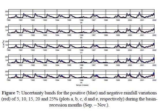
By incorporating the variations in the rainfall in accordance with Table 2, new ranges of uncertainty were estimated. To identify these new ranges and observe the differences generated by the modification of the input variables, Figures 3 to 7 show the uncertainty bands associated with the model structure and calibration parameters (white area between the black lines), the uncertainty associated with the positive variations in the rainfall (blue area), and the uncertainty associated with the negative variations in the rainfall (red area). Additionally, to quantify the propagation of rainfall uncertainty effects, Table 3 presents a summary of the average width of the uncertainty bands (in m³/s) for the different variations in the rainfall data. Additionally, Table 4 presents the percentage of variations in these ranges.

Figure 3 shows that the model outputs are sensitive to changes in the rainfall amounts, where the range of uncertainty increases by an average of 15% for positive variations and 14% for negative variations in the rainfall (Table 4). Upon comparing these results with Figure 3, it can be observed that overestimations of the rainfall amounts result in an increase in the uncertainty toward greater flows, while underestimations of the rainfall amounts result in an increase in the uncertainty of the outputs toward greater or reduced flows.

Figure 4 shows that errors in the prediction of the rainfall amounts during the winter period generate an effect on the flows of the recession curve by increasing the range of the uncertainty of the outputs of the model in the spring-summer (Oct.-Feb.) and early fall (Mar.-Apr.) (see the periods prior to the peak flows in Figure 4) and by increasing the discharge amounts estimated by the model.

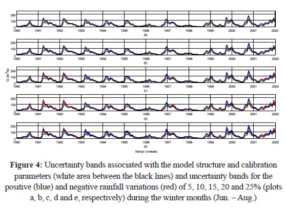
Figure 5 shows that errors in the estimation of the rainfall in summer do not significantly affect uncertainty in the model outputs, most likely because the earlier and later flows of the period mainly depend on the base flow and water storage in the basin during winter, rather than the runoff that can be produced in summer.

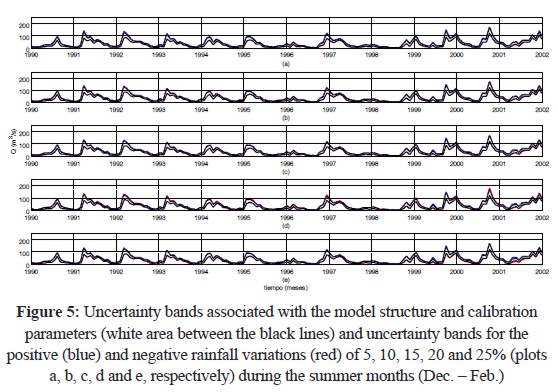
Figure 6 shows that overestimations in the prediction of the rainfall during the basin-filling period produce a displacement of the output uncertainty bands toward greater flows but maintain a relatively constant uncertainty band width (Tables 3 and 4). This result suggests that the model is highly sensitive to overestimations of the rainfall data in such a period, most likely because the model is not capable of redistributing the water in the basin processes; therefore, higher flows and similarly wide uncertainty bands are obtained. In contrast, underestimations of the rainfall in this period do not result in greater differences in the uncertainty band widths, suggesting that the uncertainty is related to different processes and/or parameters, such as the underground storage.

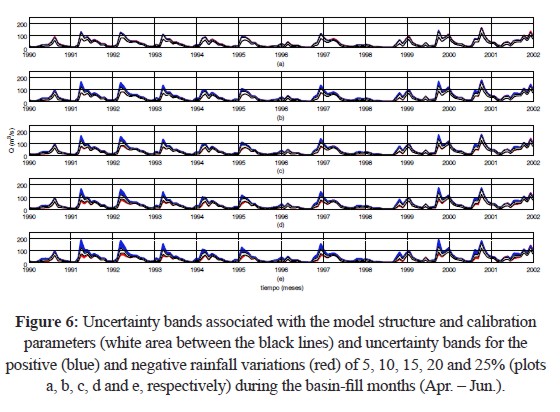
Figure 7 shows that overestimations of the rainfall in the recession period of a basin produce an increase in the output uncertainty bands, increasing the bands toward greater flows while keeping the lower limit constant.

Figures 3 to 7 show that errors in the estimation of the rainfall in a given period would affect the uncertainty in the model in subsequent periods. Additionally, errors in the estimation of the rainfall during rainy periods, especially during the filling period of the basin, generate greater uncertainty in the model outputs. This is reasonable because the greatest water intakes occur in winter, when the basin produces water storage that influences the flows of the recession curve, in addition to surface runoff. These results are also consistent with the pluvial-snow regime of the basin, in which the generated flows are directly dependent on the rainfall inputs.

Figure 7, which analyzes the influence of the rainfall in the recession period of the basin, presents similar results for the uncertainty in the estimation of the rainfall in the summer months (Figure 5); this result supports the concept of the important dependence of the model and its outputs on the inputs of water to the basin in rainy periods.

Tables 3 and 4 show that the model structure and parameters generate a 13 (m³/s) range of output uncertainty on average. After estimating how the model uncertainty is affected by uncertainty in the rainfall amounts during different periods, it is observed that the outputs are more sensitive to rainy periods. Specifically, greater ranges of uncertainty and greater percentage changes in the uncertainty bands are observed. A smaller influence is observed for low water periods (recession and summer) when the model outputs are less sensitive to errors or uncertainties in the estimation of the rainfall amounts. However, in the filling period of the basin, it is observed that the width of the uncertainty bands does not significantly increase (8% on average), but it is displaced toward greater flows when rainfall is overestimated.

CONCLUSIONS

The model is more sensitive to rainy periods; therefore, greater uncertainty in the estimation of rainfall during these periods directly influences uncertainty in the model outputs and increases the range of the related uncertainty bands.

The output uncertainty is highly sensitive to rainfall. Therefore, in dry periods, when the rainfall amounts are relatively small, the model is less sensitive to uncertainties in the rainfall than in the wet periods.

Currently, it is common to estimate flows and their uncertainty bands using a hydrological model. In the present study, it was observed that the uncertainty associated with the main water input (rainfall) in an Andean basin can generate a significant increase in the uncertainty bands of the outputs. Therefore, when using alternative sources of information to feed a hydrological model (e.g., global gridded data or data interpolated at a global scale), it is necessary to reduce the uncertainty associated with the predictions by ascertaining and reducing the deviation of the rainfall data in rainy periods (with respect to the observed or ground values) and/or by ascertaining the quality of the presented predictions. Additionally, for predictive hydrological models, high uncertainty in periods of low rainfall does not greatly influence uncertainty in the output. However, when predicting flows in rainy periods or in recession periods, the uncertainty associated with pluviometric predictability should be evaluated.

ACKNOWLEDGEMENTS

This research has been supported by the EU Erasmus Mundus External Cooperation Window, the CONICYT Programa Nacional de Formación de Capital Humano Avanzado scholarship, the BMBF/CONICYT Project 2008099 Impacto de la variabilidad climática en la disponibilidad de recursos hídricos y requerimientos de riego en la Zona Central de Chile, and the FONDECYT 11121287 project Hydrological process dynamics in Andean basins. Identifying the driving forces, and implications in model predictability and climate change impact studies. The authors thank the Dirección General de Aguas for providing the rain gauge and stream gauge data.

---

REFERENCES

Arumí, J.L., D. Rivera, E. Muñoz, M. Billib. (2012). Interacciones aguas superficiales y subterráneas en la zona central de Chile, Obras y Proyectos, 12, 4-13.

Bárdossy A. (2007). Calibration of Hydrological Model Parameters for Ungauged Catchments, Hydrology and Earth System Sciences, 11(2), 703–710.

Beven, K., and Binley, A. (1992). The future of distributed models: model calibration and uncertainty prediction, Hydrological Processes, 6, 279-298.

Caddy, J. and Mahor, R. (1995). Reference points for fisheries management. FAO Fisheries Technical Paper, 346, Food and Agriculture Organization of United Nations, Rome, Italy.

Garreaud, R. D. (2009). The Andes climate and weather, Advances in Geosciences, 22, 3–11.

Grimm, A. M., Barros, V. R., and Doyle, M. E. (2000). Climate variability in southern South America associated with El Niño and La Niña events, Journal of Climate, 13, 35-58.

Gupta, H. V., Kling, H., Yilmaz, K. K., and Martinez, G. F. (2009). Decomposition of the mean squared error and NSE performance criteria: Implications for improving hydrological modeling, Journal of Hydrology, 377, 80-91.

Mahe, G., Girard, S., New, M., Paturel, J-E., Cres, A., Dezetter, A., Dieulin, C., Boyer, J-F., Rouche, N., and Servat, E. (2008). Comparing available rainfall gridded datasets for West Africa and the impact on rainfall-runoff modelling results, the case of Burkina-Faso. Water SA, 34(5), pp. 529-536.

Montecinos, A. and Aceituno, P. (2003). Seasonality of the ENSO-related rainfall variability in central Chile and associated circulation anomalies, Journal of Climate, 16(2), 281-296.

Muñoz E. (2010). Desarrollo de un modelo hidrológico como herramienta de apoyo para la gestión del agua. Aplicación a la cuenca del río Laja, Chile. MSc. Thesis, Departamento de Ciencias y Técnicas del Agua y del Medio Ambiente, Universidad de Cantabria, España.

Muñoz, E., Rivera, D., Vergara, F., Tume, P., Arumí, JL. (2014). Identifiability analysis: towards constrained equifinality and reduced uncertainty in a conceptual model, Hydrological Sciences Journal, 59(9), 1690-1703.

Nash, J. and Sutcliffe, J. (1970). River flow forecasting through conceptual models part I: A discussion of principles, Journal of Hydrology, 10(3), 282–290.

Olsson, J., and Lindström, J. (2008). Evaluation and calibration of operational hydrological ensemble forecasts in Sweden, Journal of Hydrology, 350, 14-24.

Rango, A. and Martinec, J. (1995). Revisting the degree-day method for snowmelt computations, Journal of the American Water Resources Association, 31(4), 657-669.

SERNAGEOMIN. (2006). Mapa Geológico de Chile, Servicio Nacional de Geología y Minería, Santiago de Chile.

Vicuña, S., Garreaud, R. D., and McPhee, J. (2011). Climate change impacts on the hydrology of a snowmelt driven basin in semiarid Chile, Climatic Change, 105, 469–488.

Vörösmarty C., Fekete F., Meybeck M., and Lammers R. (2000). Global System of Rivers: It's Role in Organizing Continental Land Mass and Defining Land-to-Ocean Linkages, Global Biogeochemical Cycles, 14(2), 599–621.

Wagener, T., and Kollat, J. (2007). Numerical and visual evaluation of hydrological and environmental models using the Monte Carlo analysis toolbox, Environmental Modelling and Softwtware, 22, 1021-1033.

Wagener, T., Lees, M., and Wheater, H. (2001). A toolkit for the development and application of parsimonious hydrological models. In Singh, Frevert, and Meyer, editors, Mathematical models of small watershed hydrology, volume 2. Water Resources Publications, LLC, USA.

Willmott, C., and Matsuura, K. (2008). Terrestrial air temperature and precipitation: Monthly and annual time series (1900–2008) Version 1.02. University of Delaware Web Site, http://climate.geog.udel.edu/climate (last accessed February 2012).

Zúñiga, R., E. Muñoz, J.L. Arumí. (2012). Estudio de los Procesos Hidrológicos de la Cuenca del Río Diguillín. Análisis Mediante un Modelo Hidrológico Conceptual, Obras y Proyectos, 11, 69-78.